How I Rendered a Real-time City on Low-End Hardware: The Cost of Every Triangle and Pixel

Get the Balance Right

In this document, I wanted to share my experience working on a real-time city-rendering project and some of the optimization techniques that I believe are worth talking about.

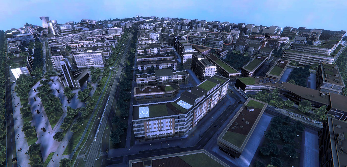
The project itself is a top-view visualization of a city sector, designed to showcase what the area may look like in the future. My role was not only to build the environment, but also to make it visually convincing and atmospheric while running in real-time.

[embed]

The biggest challenge was the target hardware.

This project was meant to run on interactive kiosk tablets, the kind usually designed for displaying documents and presentations, not large real-time rendered environments. The reference machine I used during development had an old integrated Intel GPU with extremely limited dedicated video memory, which became one of the strongest technical constraints of the entire project.

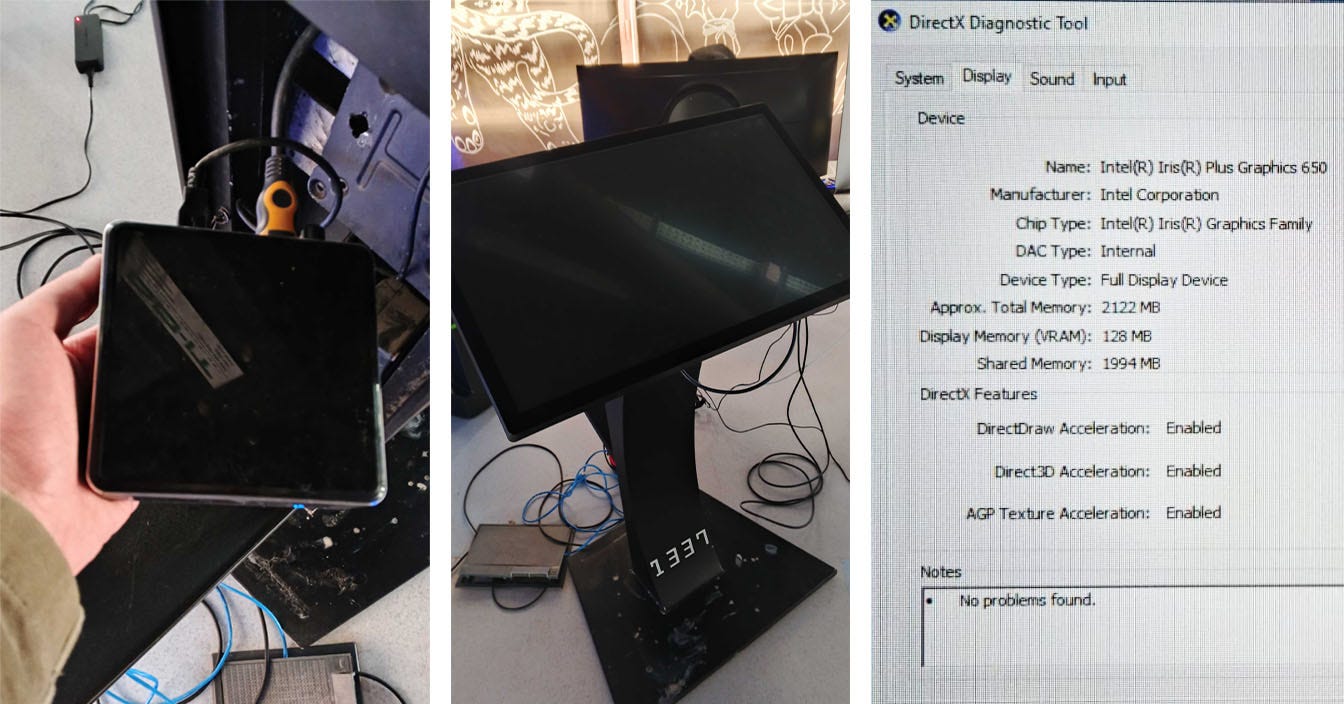
The reference machine I used

Despite those limitations, the final result was able to run at around 40–50 FPS at 1080p while still using:

• real-time lighting and shadows
• animated vegetation
• dynamic weather variations
• emissive building systems
• moving cloud shadows and reflections
• large-scale city rendering
• thousands of humans, birds, trees, and street lights

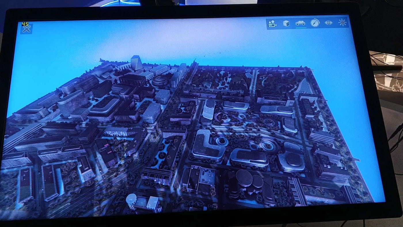
The frame rates on the reference machine

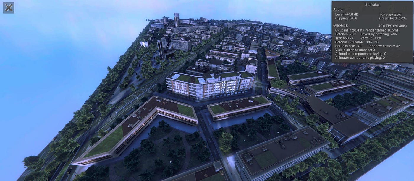
The graphic statistics from Unity

Achieving that level of performance required treating optimization as a core design principle from the very beginning rather than as a final polishing step.

Before optimizing anything, I first need to understand the nature of the project itself. The camera was positioned far above the city at roughly a 45-degree angle, meaning the environment would almost always be viewed from a distance. That completely changed the way I approached modeling, texturing, shaders, and lighting.

From that camera distance, extremely detailed geometry or high-resolution materials would provide very little visual benefit. Instead, the focus became:

• strong silhouettes
• atmosphere
• lighting
• motion
• color variation
• and carefully faked detail

The objective was not to achieve realism through brute force, but to create the illusion of richness and complexity at the lowest possible rendering cost.

Walking in My Shoes

“The purpose of painting is to decorate the walls. Therefore it has to be as rich as possible.” Pierre-Auguste Renoir

I like to think about optimization almost like a point-budget system. Every visual feature has a cost, and every project has a limited budget depending on its target hardware. The challenge is deciding where those points are worth spending.

Unlike offline media such as films or pre-rendered cinematic, real-time projects are directly constrained by performance. A movie can spend minutes or even hours rendering a single frame if needed, but a real-time application must generate dozens of frames every second while the user is interacting with it.

Because of that, visual quality in real-time graphics cannot be separated from performance. A scene may look visually impressive, but if it cannot run smoothly on its target hardware, then the experience itself begins to break down.

For that reason, I do not see optimization as a final polishing step. In real-time rendering, optimization influences nearly every artistic and technical decision from the very beginning.

Personally, I rarely like removing visual systems if they contribute to the atmosphere of a scene. Instead, I prefer understanding their rendering cost and compensating elsewhere through smarter technical decisions.

To me, optimization is not about degrading graphics in exchange for performance. If a project runs smoothly but loses its visual identity in the process, then the optimization has failed.

Another important aspect of this project was that Models, textures, shaders and code were all created from scratch. On hardware this constrained, understanding exactly where performance is being spent becomes extremely important. Building the systems myself made it easier to measure and optimize nearly every part of the rendering pipeline.

It is also important to mention that the techniques and workflows discussed throughout this document are not presented as absolute or universally correct solutions. Real-time rendering and optimization are extremely broad subjects, and there are often many different ways to solve the same problem depending on the project, hardware target, engine architecture, and production constraints.

I am still constantly learning and improving my understanding of graphics programming and real-time rendering. Many of the decisions described here were shaped by the specific limitations of this project, as well as by my own current knowledge and experience at the time of development.

In fact, this project marked my first real step into technical art. Before starting it, I did not even know technical art existed as a specialization.

My background was mostly as a generalist developer, with some web development experience and no particular focus on graphics. Around a year and half before this project, I started learning Blender, then Unity, and gradually became more interested in the technical side of real-time rendering. Many of the techniques discussed throughout this document were learned while building the project itself.

Rather than presenting this as a definitive technical guide, I simply wanted to document the approaches that worked for me throughout this project and explain the reasoning behind them.

If you are curious about some of my previous work and how I arrived at this project, you can find it on my ArtStation and LinkedIn profiles.

The following sections will break down some of the rendering techniques, optimization strategies, and technical decisions used throughout development.

Behind the Wheel

“Simplicity is the ultimate sophistication.” Leonardo da Vinci

I will start with the foundation of every 3D visual project: the models.

When people think about model optimization, the first thing that usually comes to mind is triangle count, and that is completely fair. However, there is something important that I personally overlooked when I first started working on this project.

At the time, whenever I modeled assets, I focused almost entirely on triangle count and paid very little attention to surface coverage or screen-space impact. As a result, I ended up with buildings ranging from 100 to 1000 triangles that still performed worse than significantly heavier models.

This was the moment I realized that triangle count alone is not always a reliable metric for optimization.

Before explaining why, it is important to briefly recap a few rendering concepts so the following sections make more sense.

The first thing to understand is the lifecycle of a triangle inside the rendering pipeline.

When an object is prepared for rendering, its vertex data is typically uploaded into a vertex buffer stored in VRAM. Alongside this, an index buffer defines how those vertices are connected to form triangles. Instead of resending complete geometry data every frame, the CPU mainly instructs the GPU which indices to draw, allowing the GPU to efficiently reuse existing vertex data across multiple draw calls.

The CPU then submits draw calls that tell the GPU which geometry should be rendered. From there, the GPU transforms the vertices through several coordinate spaces: object space, world space, view space, and finally screen space. At that point, the GPU knows where every triangle exists on the screen.

Next comes rasterization, where triangles are converted into fragments. A fragment contains the data required to determine how a potential pixel should be shaded.

This is, of course, an extremely simplified explanation of the rendering pipeline. Explaining every stage in detail would require an entire topic on its own.

The important part begins during fragment processing.

Before fragments are fully shaded, the GPU can perform what is commonly referred to as an Early-Z test. During this stage, fragment depth values are compared against the depth buffer before expensive fragment shader operations are executed. If a fragment is already hidden behind previously rendered geometry, the GPU can discard it early and avoid unnecessary shading work.

However, GPUs are massively parallel processors and do not always render geometry in a perfectly ordered front-to-back sequence. In many situations, fragments may still be generated and processed, before the GPU determines that they are occluded.

This leads to a phenomenon known as overdraw.

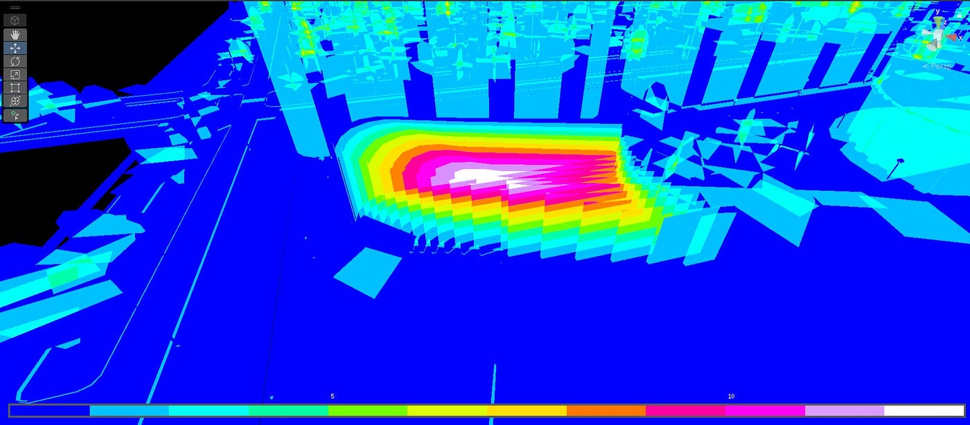
Example of severe overdraw case even if I was using opaque material

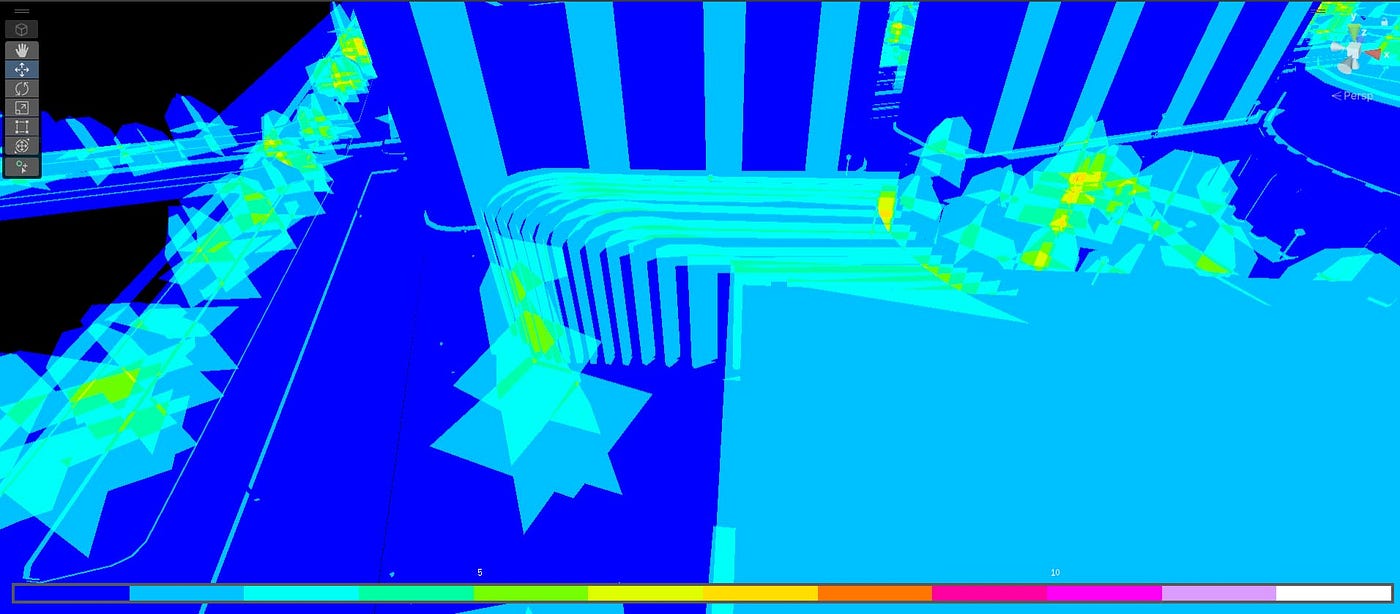
After modifying the model

Broken

Overdraw happens when multiple fragments attempt to shade the same screen pixel, even though only one of them will ultimately be visible. The discarded fragments still consume GPU resources, resulting in wasted performance.

You can think of the Early-Z test as a filtering mechanism that helps reduce unnecessary fragment shading, but cannot eliminate it entirely.

This system tends to work much better with properly separated objects, because front-to-back rendering allows nearby surfaces to populate the depth buffer earlier, making the Early-Z test significantly more effective . Unfortunately, this is something I did not fully take advantage of, since I relied heavily on chunked geometry, a design decision that I will discuss later.

Now, going back to the models.

This was exactly the problem I started noticing in some of my own models.

Large hidden surfaces, intersecting geometry, and unnecessary screen coverage were generating far more fragment work than I initially expected, even when the triangle count itself remained relatively low.

At that point, I started realizing that optimization was not only about how complex a model was in 3D space, but also about how much screen space it occupied once rendered.

Imagine we have 10 overlapping planes covering the entire screen. If we only count triangles, the cost appears very small: 2 triangles per plane multiplied by 10 gives us only 20 triangles total.

At first glance, that sounds almost free from a rendering perspective.

However, if those planes cover a full 1080p display, the GPU may still end up generating and processing millions of fragments. A single 1080p frame contains over 2 million pixels, and with 10 full screen overlapping layers, the fragment workload can increase dramatically if overdraw occurs and the Early-Z test cannot reject enough hidden fragments efficiently.

So while the triangle count remains very low, the fragment shading workload becomes enormous, and that is where the real performance bottleneck begins to appear.

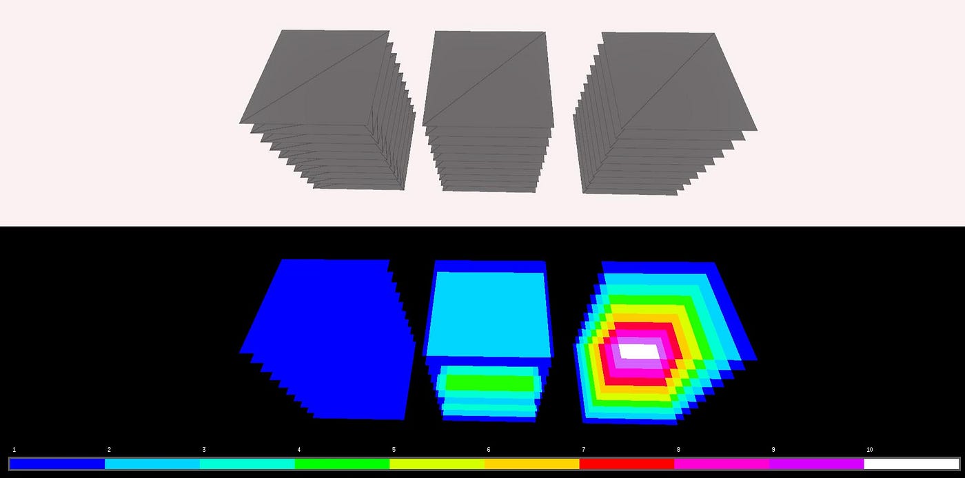
Triangle count, draw calls and overdraw are often competing costs.

All three examples represent ten overlapping surfaces, but each approaches the problem differently.

The first version merges the geometry into a single object with no additional cuts. This results in very few triangles, but produces severe overdraw because large hidden regions are still rasterized.

The second version keeps each surface as a separate object. This increases object count and rendering overhead, while overdraw remains relatively high.

The third version removes the hidden portions of the geometry entirely. This significantly reduces overdraw, but requires many more triangles to describe the visible shape.

None of these solutions is universally correct. The optimal choice depends on whether the bottleneck is vertex processing, fragment shading, memory bandwidth, or CPU overhead. The important lesson is that reducing triangle count alone does not necessarily produce the fastest result.

Cover me

“Art is the elimination of the unnecessary.” Pablo Picasso

Naturally, every model also requires its own textures and materials.

At this stage, the challenge was no longer limited to reducing polygon counts, but also reducing how much data the GPU constantly needed to manage and access during rendering.

One of the first principles I try to keep in mind is simply: avoid forcing the GPU to change state too frequently. GPUs are designed to perform extremely efficiently when executing the same type of workload repeatedly. Interrupting that flow introduces what is commonly referred to as a state change.

A state change can occur when switching:

• shaders
• materials
• textures
• render states
• or even different rendering configurations between objects

While a single state change may appear inexpensive, thousands of them across an entire scene can quickly become a significant performance cost.

Textures themselves are essentially data describing the visual properties of a surface, and like any form of data, they also need to be optimized.

In theory, every surface in a scene could use its own unique high-resolution texture set along with dedicated material masks and detail maps. In practice, however, this introduces substantial memory and bandwidth overhead very quickly.

One thing that is particularly easy to underestimate is how aggressively textures can consume VRAM when they are not managed properly.

Take a simple building surface as an example.

You may begin with a 1024×1024 albedo texture. Then add:

• a roughness map
• a metallic map
• a normal map
• and perhaps an emissive mask

On top of that, each texture also requires mipmaps. If all of these textures are stored carelessly using uncompressed RGBA32 formats, memory usage can rapidly grow into tens of megabytes for a single material on a single building.

And that is before considering the rest of the scene.

Because of this, texture optimization must account for several factors simultaneously:

• texture resolution
• GPU storage format
• channel usage
• compression methods
• the number of textures simultaneously resident in VRAM
• texture streaming behavior
• and total texture bandwidth during rendering

It is important to clarify that optimization here is not about the PNG or JPEG file size stored on disk. What truly matters is the decompressed texture format the GPU ultimately stores and samples in memory.

Smaller reusable textures also improved texture cache locality and reduced bandwidth pressure compared to constantly sampling large unique texture sets.

To solve these problems, there are many possible approaches. In this project, I primarily combined texture atlasing with tiled materials.

Precious

Atlasing is the process of packing multiple surface types into a single texture. Tiling, on the other hand, is a technique where a texture repeats seamlessly across a surface, allowing relatively small textures to cover very large areas.

Like every optimization technique, both approaches come with their own trade-offs.

With atlasing, one of the main compromises is memory efficiency. Because multiple surface types are packed into a single large texture, the GPU must keep the entire atlas resident in VRAM even if only a small portion of it is actually being used by the current scene.

For example, imagine an atlas containing textures for a tree, a car, a boat, and a dog. If the scene only contains the tree and the car, the GPU still needs to keep the complete atlas loaded in memory, including the unused boat and dog regions. In practice, this means a potentially large percentage of texture memory may be occupied by data that contributes nothing to the final image.

In many projects, this can become inefficient. However, in this particular case, atlasing worked extremely well because the assets were designed in a way where most atlas regions were consistently reused throughout the entire environment. This minimized wasted texture space while still reducing material and texture switches.

Using atlasing alone would eventually have made surface variety increasingly expensive. Every surface type needs to occupy space inside the atlas, and once that space became limited, I would have been forced to split geometry into additional surface regions and UV layouts to fit everything. On the other hand, relying entirely on tiled materials would have required many additional texture sets and material instances, increasing both texture switches and overall material complexity.

So instead, I combined both approaches.

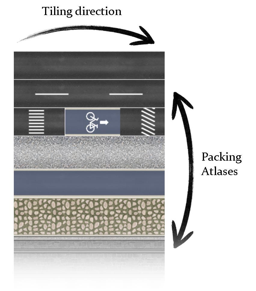
Horizontally, textures are tiled across surfaces, allowing relatively small texture regions to repeat seamlessly over large geometry. Vertically, multiple surface types are packed together inside shared atlases. This hybrid workflow allowed me to preserve visual variation while still minimizing texture count, memory pressure, and material complexity.

Another major advantage of this workflow was organization.

Because the surfaces were centralized into structured atlases rather than scattered across hundreds of unrelated texture sets and UV layouts, editing became significantly easier to manage. Adjusting masks, tweaking material properties, or introducing additional surface variations could all be done in a far more controlled and scalable way.

In the end, nearly 90% of the entire project relied on only two primary texture sets:

• one atlas dedicated to buildings
• and another dedicated to infrastructure and environmental surfaces

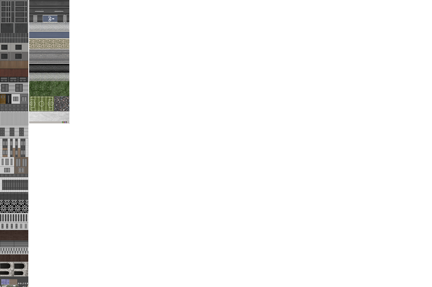
The two albedo textures used in the two main materials

It’s No Good

Now you have built your shaders and material set. You can finally view your buildings in full color, with convincing lighting, reflective surfaces, and atmospheric detail.

Then you run the project… and performance is far worse than expected.

At that point, you quickly realize there are still many things being overlooked.

One of the core principles I always try to follow is this: never perform calculations in a shader if they can be avoided entirely or moved to a cheaper stage of the pipeline.

Take a simple example.

If you look closely at the building surfaces, many areas contain windows, reflections, and higher-detail materials. However, a large portion of the geometry is actually made up of flat, single-color surfaces with very little visual complexity.

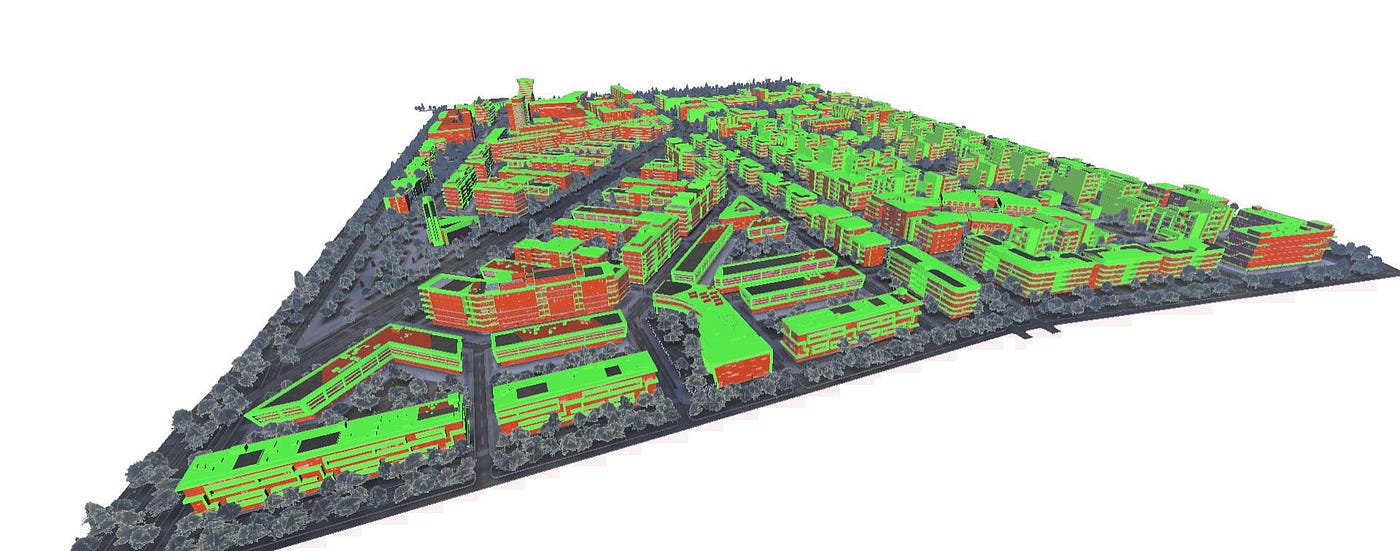
Green surfaces are using cheaper shader from the red surfaces

Despite that, the exact same expensive shader was still being executed across every surface.

Naturally, this felt wasteful.

My first instinct is usually to introduce branching to skip expensive features on simpler surfaces. But after testing, performance barely changes, even after skipping most shader features.

This is where it becomes important to understand how GPUs actually execute shaders.

Shaders are not executed like traditional CPU code with highly dynamic branching and intelligent decision-making. Instead, GPUs execute instructions massively in parallel across many fragments simultaneously.

Because of this, conditional branching inside shaders does not always remove the underlying cost. Depending on shader divergence, execution grouping, and compiler behavior, the GPU may still execute large portions of both code paths internally.

As a result, simply “turning off” features inside a single monolithic shader often provides far less benefit than expected.

In many situations, the better solution is to create separate shader variants that completely remove unnecessary calculations for specific material categories.

Hole to Feed

“Perfection is achieved, not when there is nothing more to add, but when there is nothing left to take away.” Antoine de Saint-Exupéry

In my case, one of the first optimizations I introduced was removing texture sampling entirely from simplified shader variants.

Many surfaces were nothing more than flat colors. Sampling textures, which is relatively expensive compared to simple arithmetic or interpolated vertex data, was completely unnecessary.

Instead, I replaced those texture lookups with a much cheaper source of information: vertex attributes.

Each vertex can store additional data, including vertex color values. By baking flat color information directly into the mesh itself, I could eliminate texture fetches entirely for many surfaces.

Another optimization involved storing lightweight material information directly inside secondary UV coordinates instead of relying on additional mask textures.

Every vertex already contains UV coordinate data (u, v), so I repurposed part of that existing data to carry simplified material information.

For example, if I wanted a portion of a mesh to behave as a reflective surface, I could place those vertices at a specific coordinate inside a secondary UV channel. A coordinate such as (0.5, 0) could later be interpreted inside the shader, where the U component becomes a smoothness value or material mask.

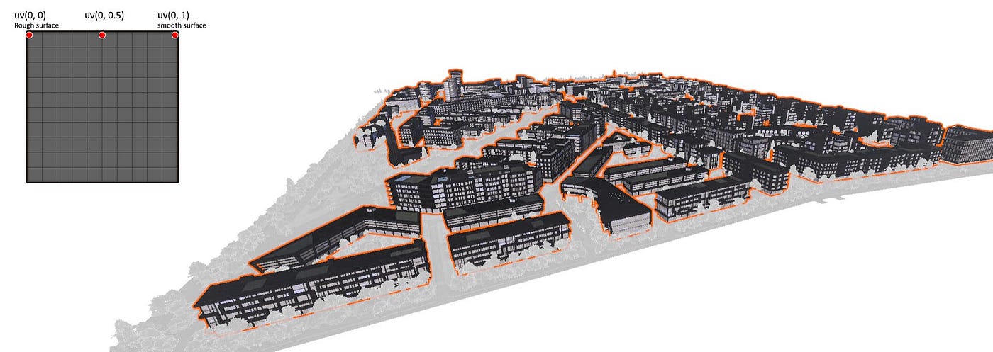
White surface is smooth as for black is rough (visualizing buildings only)

In practice, this meant the mesh geometry itself was carrying lightweight material information.

Instead of sampling extra mask textures to determine whether a surface should be reflective, emissive, or excluded from certain effects, the shader could simply read values already embedded inside the vertex data.

One final thing worth mentioning is that I almost always avoid procedural noise functions whenever possible.

Instead, I rely heavily on extremely small precomputed noise textures tiled across surfaces.

Procedural noise is generated mathematically inside the shader itself, and while modern GPUs can handle it reasonably well, the cost can still become significant when evaluated across large screen regions and millions of fragments simultaneously.

In my particular case, I simply did not need that level of procedural complexity.

Most of the time, the noise was not being enlarged to generate meaningful close-up detail. Instead, it was simply repeated across distant surfaces viewed from a high-altitude camera angle.

At that scale, a tiny tiled noise texture became visually almost indistinguishable from procedural noise while being dramatically cheaper to evaluate.

So instead of paying the cost of per-fragment procedural calculations, I achieved nearly the same visual result using a single inexpensive texture sample.

Sibeling

Alongside GPU optimization, the CPU side also needs to be managed carefully so it does not become a bottleneck itself. Even if the GPU is capable of rendering frames quickly, the entire pipeline can still stall if the CPU cannot prepare rendering commands fast enough.

In real-time rendering, performance is never determined by the GPU alone. The CPU and GPU operate as a pipeline, and both sides must remain balanced to maintain stable frame times.

Now let us go back to the models.

Another optimization technique I relied on heavily throughout the project was chunking. This approach helped address two major problems simultaneously:

• reducing draw calls
• improving culling efficiency

One of the largest CPU-side challenges in real-time rendering, even on relatively powerful hardware, is the sheer number of draw calls submitted every frame. The CPU can quickly become overwhelmed by the amount of rendering work it needs to prepare and send to the GPU.

A draw call is essentially an instruction telling the GPU to render a batch of geometry.

That batch can represent many different things:

• a single tree
• multiple trees
• a building
• a UI element
• a skybox
• or even thousands of repeated objects

In practice, every time the rendering state changes, a new draw call is usually required.

This means even relatively simple scenes can generate surprisingly high draw call counts if assets and materials are not organized carefully.

One common technique used to reduce draw calls is static batching.

Static batching works by combining multiple objects into a single larger mesh so they can be rendered together using fewer draw calls.

This approach also introduces several important trade-offs.

The first limitation is that the geometry can no longer move independently after being merged. For my use case, this was perfectly acceptable.

The second limitation, however, was far more problematic.

Once large amounts of geometry are merged into a single mesh, culling becomes significantly less efficient.

Frustum culling works by skipping objects outside the camera view, preventing unnecessary rendering work. But if an entire city block becomes one massive combined mesh, then as long as even a small portion of that mesh remains visible, the renderer may still need to process the entire object.

In my case, that would have resulted in large sections of the city continuing to move through the rendering pipeline even when most of their geometry was completely outside the camera view.

This is where chunking became a much more balanced solution.

Instead of merging the entire city into a few enormous meshes, I manually grouped buildings and environmental assets into smaller chunks inside Blender. Each chunk contained multiple merged objects, allowing several buildings to be rendered together in a single draw call while still preserving reasonably effective frustum culling.

As a result:

• the CPU had significantly fewer draw calls to submit
• while the renderer could still discard entire chunks outside the camera view

This created a much better balance between CPU overhead and culling granularity.

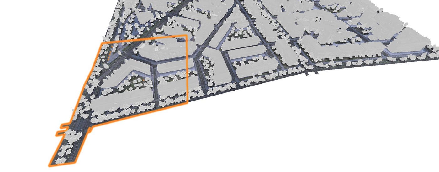
Example of a chunk (1 of 15 ground chunks)

Of course, chunking also introduced its own drawbacks.

Ghosts Again

Earlier in the document, I mentioned how Early-Z rejection works more effectively when geometry is separated cleanly and rendered in a front-to-back order. Because my chunks contained many merged objects, hidden geometry inside a chunk could still generate unnecessary fragment work before eventually being rejected by depth testing. In other words, I reduced CPU overhead at the cost of introducing additional overdraw on the GPU side.

This became one of the recurring themes throughout the entire project: Most optimization techniques are not universally “good” or “bad.” They are trade-offs. The real objective is deciding which trade-offs are the most acceptable for the target hardware, rendering constraints, and visual goals of the project.

Chunking was one of the primary techniques I used to reduce CPU-side rendering overhead, but it was not the only one. Another major source of CPU cost came from the large number of repeated objects scattered throughout the city. Even if individual assets were lightweight, rendering thousands of copies still required the CPU to prepare and submit a significant amount of work.

This is where instancing became extremely valuable.

I primarily used instancing for assets that were repeated heavily across the city, such as:

• trees
• humans
• cars
• light poles
• birds

Instancing works by rendering many copies of the same mesh using a single draw call. Instead of repeatedly sending duplicate geometry data to the GPU, the CPU submits the mesh once alongside an array of per-instance transform data describing the position, rotation, and scale of each copy.

This dramatically reduces CPU overhead because the GPU can render large numbers of identical objects without requiring separate draw calls for every individual instance.

However, instancing also comes with important restrictions.

All instances generally need to share:

• the same mesh
• the same material
• and the same shader configuration

It also becomes less suitable for objects requiring unique deformation or complex animation, especially skinned meshes using skeletal animation, where every object may require its own vertex transformations and animation state.

For moving objects such as trees, I relied heavily on vertex shader animation, which works exceptionally well alongside instancing while remaining extremely lightweight.

Instead of using skeletal animation or expensive simulation systems, the movement is generated directly inside the vertex shader by applying controlled procedural offsets to the vertex positions. This allows the geometry to sway and deform in a believable way, creating the illusion of wind and moving foliage at a very low rendering cost.

Because the animation happens entirely on the GPU and does not require unique mesh data per object, the vegetation can still fully benefit from instancing. This allowed large numbers of animated trees to exist simultaneously without introducing significant CPU overhead or additional draw calls.

People Are People

“Art is not what you see, but what you make others see.” Edgar Degas

Another type of asset where I relied heavily on vertex shader animation was the pedestrians throughout the city.

The scene contains hundreds of people visible at the same time. If every character used a fully skinned mesh with independent skeletal animation, the performance cost would increase dramatically on both the CPU and GPU sides.

Even modern games still struggle with rendering and animating very large crowds efficiently. At a certain scale, fully simulated skeletal animation simply becomes too expensive relative to the visual benefit, especially for distant characters viewed from a high camera angle.

Traditional skeletal animation works by assigning every vertex one or more bone weights describing how strongly that vertex is influenced by different bones in the skeleton. During animation, the GPU (or sometimes CPU) must continuously transform and blend those vertices using multiple bone matrices every frame.

For a single character, this is perfectly reasonable.

For hundreds of distant background pedestrians, however, the cost quickly becomes difficult to justify.

In my case, the characters were almost always viewed from far away, meaning the animation only needed to communicate one thing convincingly: the illusion of motion.

At that distance, a believable walking cycle can be reduced to three essential visual cues:

• limb movement
• mirrored limb timing
• and vertical body motion

That alone is often enough for the brain to interpret a character as walking.

So instead of using skeletal rigs, I created an extremely lightweight procedural animation system directly inside the vertex shader.

To animate the limbs, I needed a way to identify which vertices belonged to specific body parts and how strongly they should move. I used the UV coordinates of the mesh itself to encode that information.

To animate the limbs, I needed a lightweight way to identify both:

• which side of the body a vertex belonged to
• and how strongly that vertex should move

I encoded both pieces of information directly into the mesh UV coordinates.

The U coordinate was used as a simple left/right mask. Vertices belonging to one side of the body were assigned a value of 0, while the opposite side received a value of 1.

This allowed the shader to distinguish between left and right limbs and automatically mirror their movement by applying opposite animation phases.

The V coordinate was then used to control movement intensity along the limb itself.

For example, vertices near the shoulder could receive a value close to 0, while vertices near the hand would receive values closer to 1. The shader could then use this gradient to smoothly interpolate the amount of movement across the limb.

As a result:

• the shoulder remained relatively stable
• while the hand and lower arm swung much more aggressively

This created a simple but convincing approximation of limb rotation entirely through vertex deformation, without requiring skeletal animation or bone weights.

Finally, the overall body movement was completed by applying a subtle vertical offset to the entire mesh, creating the bouncing motion associated with walking.

The final result was an extremely cheap animation system capable of animating large crowds simultaneously while remaining fully compatible with instancing.

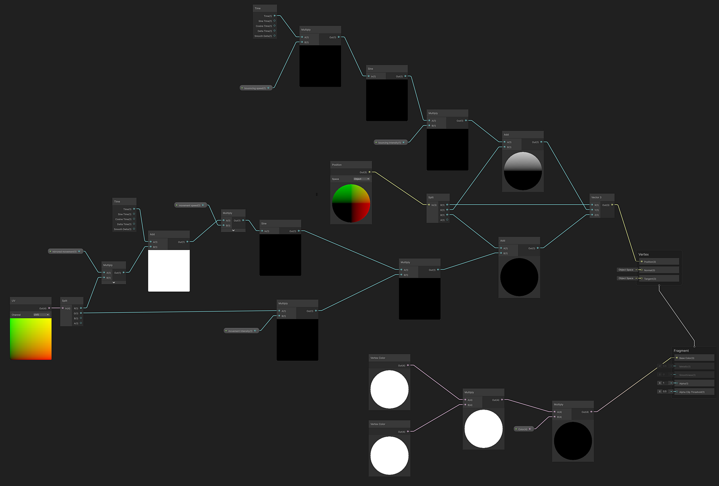
The full shaderGraph of pedestrians

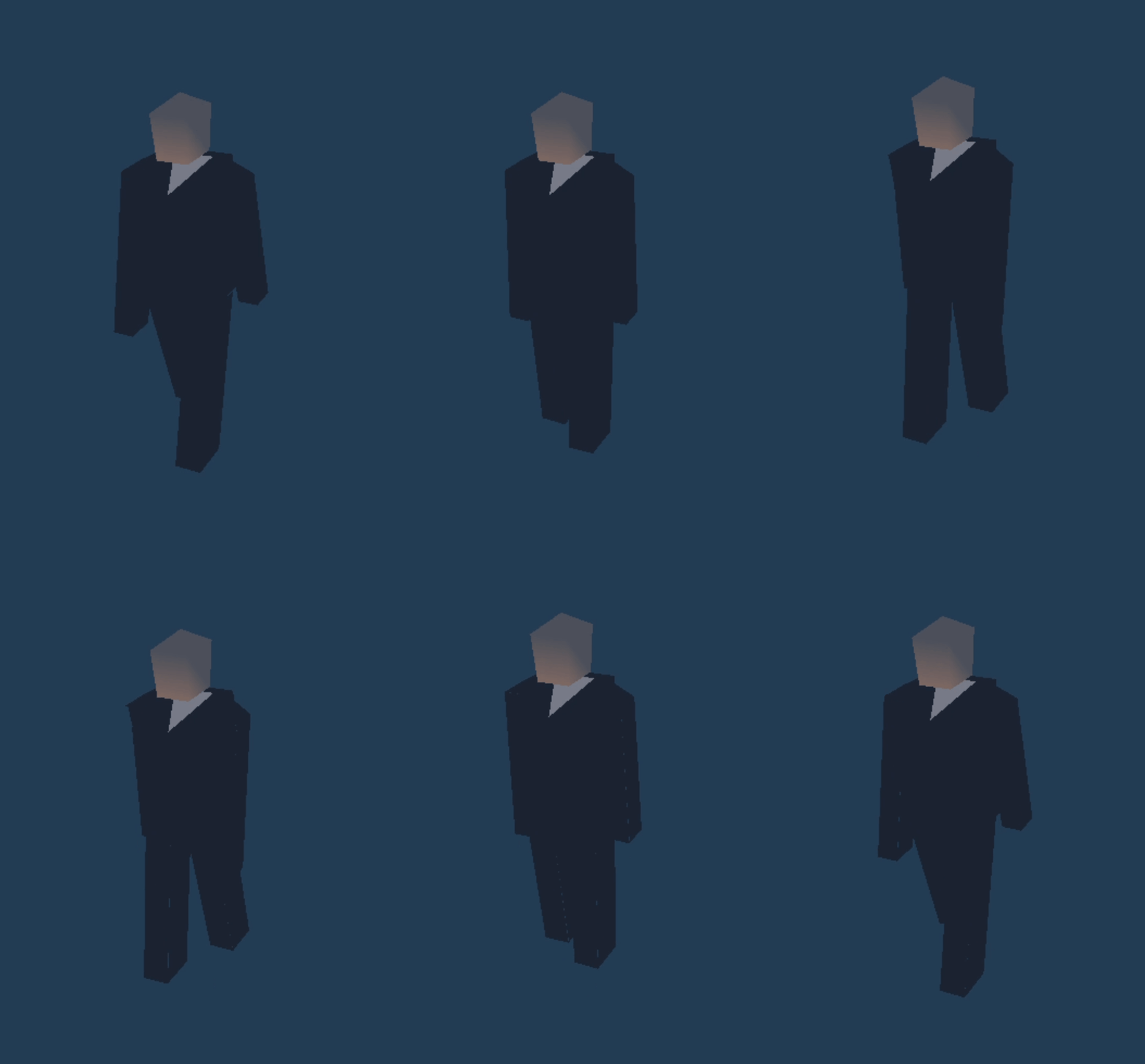
fully animated pedestrian with only 60 triangles

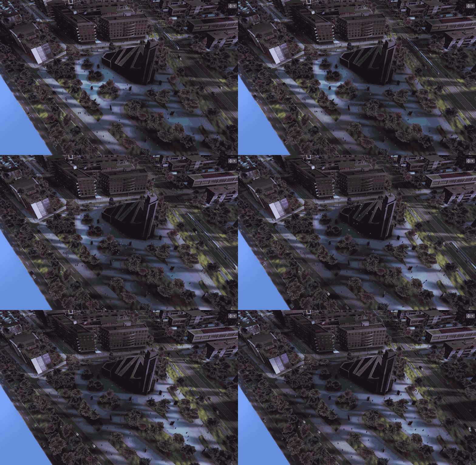
I applied a very similar idea to the birds in the scene.

The birds are intentionally extremely simple, essentially just two animated triangles representing flapping wings viewed from a distance.

However, unlike the pedestrians, part of the bird movement logic was moved to the CPU instead of being calculated entirely inside the vertex shader. This allowed certain shared motion calculations to be performed once on the CPU rather than repeatedly per vertex across every bird instance.

At the scale and viewing distance used in the project, this approach produced a convincing illusion of motion at an extremely low rendering cost.

Fragile Tension

“Nature is pleased with simplicity.” Isaac Newton

Trees are always one of the parts that make me the most nervous when starting a project, because vegetation is notoriously one of the hardest things to optimize in real-time rendering.

The main reason for this is alpha-clipped foliage.

When rendering a tree, the obvious challenge is the sheer amount of geometric detail involved. A real tree contains thousands upon thousands of individual leaves, and representing all of them using actual geometry would destroy performance almost immediately.

To solve this, most real-time projects rely on foliage cards.

Instead of modeling every individual leaf, multiple leaves are packed into a single texture containing an alpha mask, then mapped onto simple polygon planes. A single card can represent dozens of leaves at once, reducing the geometry from potentially tens of thousands of polygons down to only a few triangles.

At first glance, this sounds like an excellent optimization technique, and in many ways, it is.

However, it also introduces another major problem: overdraw.

Earlier in the document, I explained how the Early-Z test attempts to reject hidden fragments before expensive fragment shading occurs. Unfortunately, alpha-clipped geometry interacts very poorly with this process.

The reason is that during the Early-Z stage, the GPU only sees the raw polygon geometry itself. At that point, the renderer still does not know which parts of the texture will later be discarded by the alpha mask.

The fragment shader must first evaluate the alpha value before determining whether that fragment should remain visible or be clipped away.

Because of this, alpha-clipped surfaces often reduce the effectiveness of Early-Z rejection and can prevent depth information from being written as efficiently as fully opaque geometry.

The result is extremely high overdraw.

If a tree contains dozens or even hundreds of overlapping foliage cards, the GPU may repeatedly process the same screen pixels many times before final visibility is resolved.

In dense vegetation scenes, this can become enormously expensive very quickly.

This is one of the reasons vegetation often becomes one of the heaviest rendering costs in large outdoor scenes despite appearing deceptively lightweight in terms of triangle count.

Policy of Truth

“Reality leaves a lot to the imagination.” John Lennon

Fortunately, my project had one very important advantage.

Since the entire experience is viewed from a distant top-down perspective, I did not actually need dense foliage geometry or highly volumetric trees. What I really needed were convincing silhouettes.

Because of that, the trees are surprisingly simple. Most of them are constructed from only three or four intersecting foliage cards, with variation introduced through scaling, rotation, and slight shape differences.

Naturally, this raises an obvious concern:

Wouldn’t the trees look flat?

And honestly, under traditional lighting, they absolutely would.

But this led to one of the most interesting visual decisions in the entire project.

Sometimes optimization removes visual quality. Sometimes optimization preserves visual quality. And occasionally, optimization actually improves the final image.

In this case, I realized that realistic lighting was actually making the trees look worse.

Because the foliage consisted of only a few intersecting cards, traditional lighting exposed the underlying structure too clearly. Directional lighting and specular highlights revealed the flat surfaces that the foliage illusion was trying to hide.

The more physically accurate the lighting became, the more obvious the trick was.

So instead, I moved toward an entirely unlit foliage shader.

Rather than responding to scene lighting, the trees preserve their own shading and color information, almost like stylized sprites placed directly into the environment. This allows the silhouettes to remain readable while helping conceal the card structure itself.

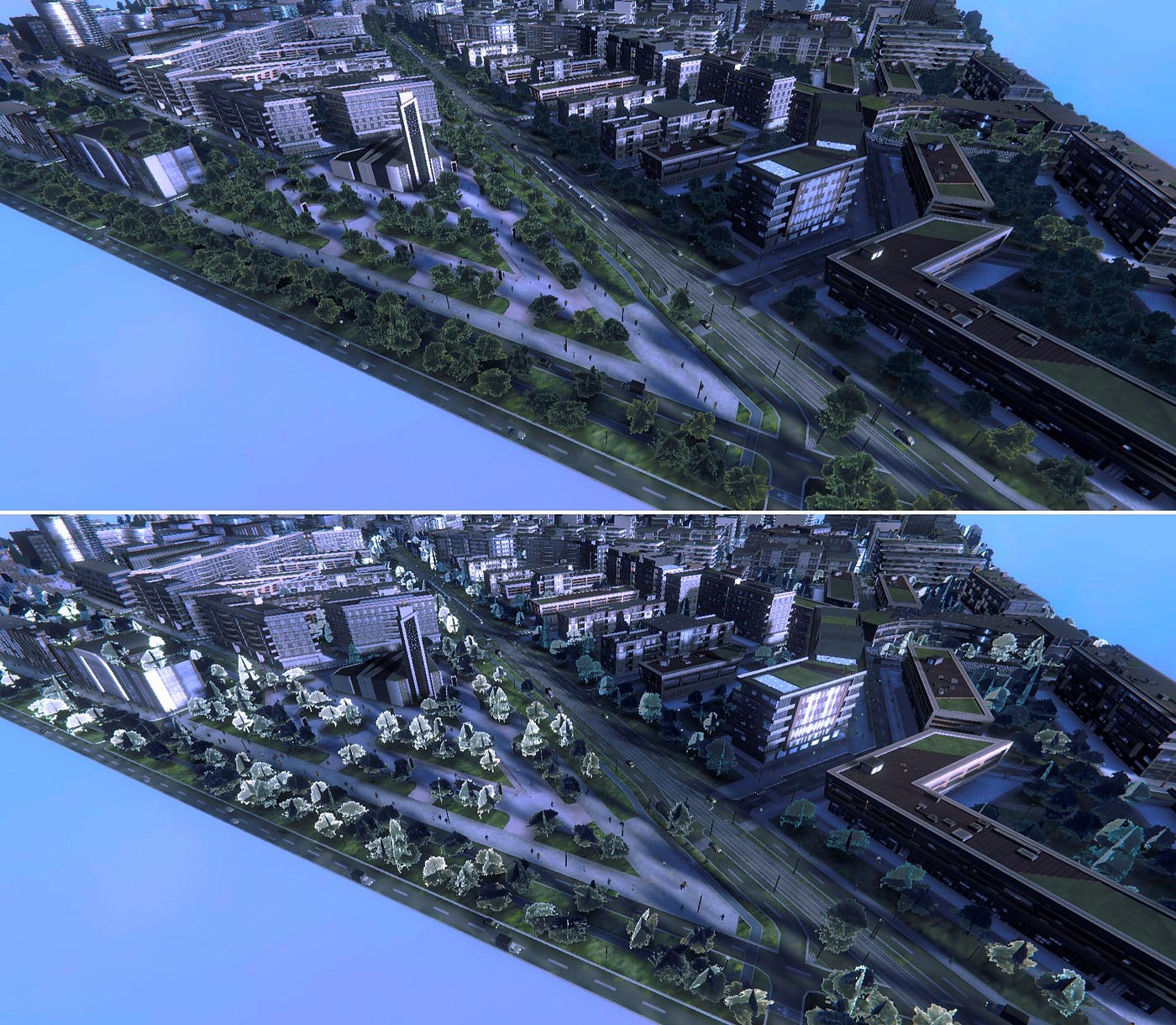
Unlit against Lit trees shader

Ironically, the simplified shader not only became significantly cheaper to render, but also produced a more convincing result from the project’s camera distance.

As a result, I could populate the city with significantly more vegetation without constantly worrying about performance costs.

In this particular case, reducing realism actually improved both performance and visual quality at the same time.

I should also mention that vegetation relied heavily on material LODs.

Wrong

Normally, when people talk about LODs, they are referring to mesh complexity, where distant objects are replaced by lower-polygon versions. However, LOD systems can also be applied to materials and shaders.

Because the foliage shader was unlit, distant trees did not naturally integrate with atmospheric effects such as fog. Without additional processing, they began to appear visually disconnected from the environment, almost as if they were floating on top of the scene.

To solve this, I introduced a simplified distance-based fog calculation directly into the trees shader. As trees move farther away from the camera, they gradually blend toward the atmospheric fog color, helping them integrate more naturally into the environment.

This also created the perfect opportunity for material LOD transitions.

Once distant trees became heavily obscured by fog, individual leaf shapes were no longer distinguishable. At that point, I could safely swap them to even cheaper shader variants that no longer relied on alpha clipping.

Because the transition occurred inside dense fog, the visual difference was largely hidden, making the LOD change almost impossible to notice.

To manage this efficiently, the vegetation was organized into spatial chunks that were precomputed during scene initialization. This allowed entire groups of trees to transition between material LODs together based on camera distance while keeping CPU overhead extremely low.

As for shadows, I chose a different approach entirely.

Rather than having vegetation fully participate in dynamic shadow receiving, I approximated the shadow response through shader parameters.

Trees were organized into groups based on whether they occupied predominantly shadowed or illuminated areas of the environment. These groups could then receive different shading parameters without requiring separate materials.

To modify those values efficiently, I relied on Material Property Blocks.

Material Property Blocks allow per-renderer shader parameters to be modified without creating additional material instances. This made it possible to adjust properties such as color tinting while continuing to reuse the same underlying material.

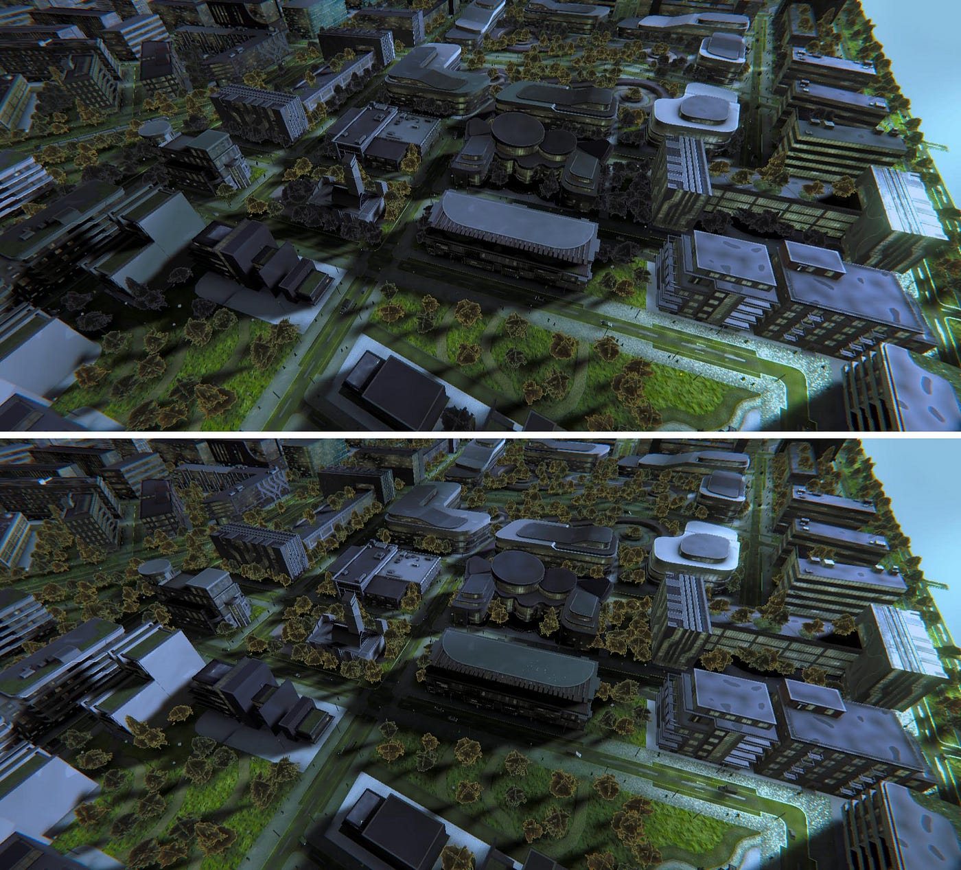
With / without faking received shadows on trees

This was important because creating large numbers of unique material instances can increase memory usage and reduce rendering efficiency. By using Material Property Blocks, I could introduce visual variation while preserving the benefits of shared materials.

Just Can’t Get Enough

“In nature, light creates the color. In the picture, color creates the light.” Hans Hofmann

Lighting is the backbone of almost every visual project.

It can elevate a scene dramatically, or completely undermine its atmosphere if handled poorly. At the same time, lighting is also one of the most expensive systems in real-time rendering, making it especially important to approach it carefully.

Personally, lighting is the area where I try the hardest not to compromise visually.

I would rather aggressively optimize almost every other aspect of the project so that I can preserve enough performance budget to work more freely with lighting, atmosphere, and overall mood.

If you look closely at the buildings in the project, one thing you will immediately notice is the strong reflection highlights visible on the windows.

Interestingly, those reflections are not physically accurate at all.

Based on the actual position of the directional sunlight, many of those highlights would not realistically be visible from the camera angle being used. The viewing direction and reflection vectors simply would not align in a way that produces those reflections.

However, from a visual perspective, the reflections contributed enormously to the readability of the city.

So instead of pursuing physical accuracy, I introduced a secondary artificial light source used exclusively for window reflections.

Its sole purpose was to generate readable highlights on the glass surfaces and enhance material variation across the buildings.

The result was a city that appeared significantly richer and more detailed from a distance, particularly while the camera was moving, where the reflections helped separate building forms and reinforce surface variation.

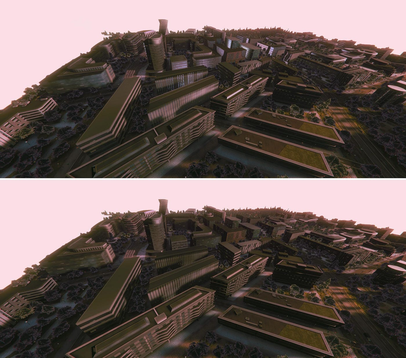
With/without the fake light reflections

To keep this efficient, both the reflective materials and the secondary reflection light were isolated using rendering layers. This ensured that the additional lighting calculations only affected the building glass rather than the entire scene.

Another effect that contributed heavily to the atmosphere was the movement of cloud shadows and cloud reflections across the city.

Of course, I was not rendering actual volumetric clouds, nor was I projecting real cloud shadows onto the environment.

Instead, I introduced animated masks directly into the shaders responsible for rendering the city.

In reality, both effects are little more than controlled animated gradients and color modulation.

However, because the building and infrastructure shaders already occupy the vast majority of the visible screen space, affecting only those two materials was enough to make the entire city appear influenced by changing cloud cover.

The technique was extremely inexpensive while adding a surprising amount of movement, scale, and atmosphere to the environment.

Lighting became even more important during nighttime scenes.

I relied heavily on localized lighting to shape the atmosphere after dark. Pools of light helped guide attention, define streets, and create visual contrast throughout the city.

While non-shadow-casting lights are significantly cheaper than dynamic shadow-casting lights, they can still become expensive when large numbers of them overlap.

Every additional light potentially increases the amount of lighting work that must be performed, particularly when many objects fall within the influence of multiple lights simultaneously.

Heaven

Lighting accumulation introduces its own challenges.

In a traditional forward rendering pipeline, every light affecting a surface may require additional lighting calculations during the shading process. As more lights overlap, the amount of work performed per pixel can increase significantly.

And honestly, even the “fake” reflection system was more excessive than I initially admitted.

In reality, I ended up using two separate artificial reflection lights depending on the orientation of the buildings. Different facade directions received different highlight sources to maintain strong readability across the city.

At some point, you begin to realize something funny about real-time lighting: You almost never feel like you have enough of it.

This is one of the reasons many modern rendering pipelines rely on deferred rendering when dealing with large numbers of dynamic lights.

The core idea behind deferred rendering is to separate geometry rendering from lighting calculations.

Instead of calculating lighting immediately while rendering geometry, the renderer first stores surface information such as normals, material properties, and depth into a set of intermediate buffers commonly known as the G-buffer.

Once this information has been collected, lighting is evaluated as a separate pass using the data already stored in those buffers.

This can become significantly more efficient in scenes containing many overlapping lights because geometry is shaded only once during the geometry pass, while lighting is accumulated afterward using the information stored in the G-buffer.

However, deferred rendering also comes with important costs.

The G-buffer requires several additional render targets to store all of this intermediate data, increasing both memory usage and memory bandwidth requirements.

For my target hardware, this was simply not a realistic option.

The development machine relied on an older integrated Intel GPU with extremely limited available video memory. Under those constraints, allocating multiple full-screen render targets for a deferred renderer would have consumed a substantial portion of the available memory budget before considering textures, shadow maps, or any other rendering resources.

This is one of the reasons deferred rendering is often avoided on lower-end or memory-constrained hardware, where memory bandwidth and render target storage can become major bottlenecks.

Because of that, I stayed entirely with a forward rendering approach and focused instead on carefully controlling where and how lighting was applied.

A Question of Time

Another possibility would have been fully baked lighting.

However, baking lighting for an entire city would also introduce significant costs of its own.

Maintaining consistent visual quality across such a large environment would require very large lightmaps. This would place considerable pressure on the available memory budget.

For a project targeting extremely constrained hardware, this quickly becomes a concern.

So instead of baking the entire lighting solution, I chose to bake only the ambient occlusion.

Ambient occlusion was one of the more expensive visual effects in the project, particularly given the scale of the environment and the amount of visible geometry present throughout the city. Baking it allowed me to preserve much of the grounding, contact shadowing, and depth perception it provides without paying the runtime cost continuously.

The process itself was far from simple.

I manually prepared secondary UV layouts for the assets inside Blender, carefully allocating texel density based on how visible different surfaces would be from the project’s camera angle.

Areas that were frequently visible received a larger share of the available texture space, while less important surfaces were intentionally given lower priority to conserve memory.

Alongside ambient occlusion, I also baked cavity information because it contributed significantly to the perceived depth and material definition of the environment.

This became especially valuable from the project’s distant camera perspective, where subtle shading cues often communicate more visual information than geometric detail.

This highlights another side of optimization that is not discussed nearly as often: the human cost.

Many optimization techniques do not only affect visual fidelity.

They also affect development time, workflow flexibility, iteration speed, and creative freedom.

Some techniques are extremely efficient from a rendering perspective but introduce additional complexity into the production process.

For that reason, I generally avoid heavily baked workflows unless the performance benefits clearly justify the additional production cost.

Tora! Tora! Tora!

And for every light come the shadows, and shadows introduce their own significant performance cost.

Real-time shadows are expensive because the renderer must effectively render the scene again from the perspective of the light in order to determine which areas are occluded. This process is commonly referred to as the shadow pass.

During this pass, the CPU still needs to submit draw calls for every object configured to cast shadows. The GPU then processes the geometry through the vertex stage and rasterization stage in order to generate the shadow map.

Fortunately, shadow rendering is usually cheaper than the main rendering pass because it often avoids many of the expensive fragment shading operations used during final surface rendering. In most cases, the renderer primarily cares about depth information rather than complete material evaluation.

Even so, shadow rendering can still become extremely expensive when large amounts of geometry participate in the shadow pass.

Because of that, one of the most effective ways to optimize shadows is reducing the geometric complexity of the objects casting them.

However, simply lowering the triangle count of every visible asset is not always a good solution, since it may visibly damage the final image quality.

Instead, I relied heavily on shadow proxies.

A shadow proxy is a simplified invisible mesh used exclusively for shadow casting. The visible object remains visually detailed, while a much cheaper hidden mesh is responsible for generating the shadow silhouette.

This can reduce shadow rendering cost dramatically.

For example, my trees shadow proxies were reduced to two triangles, as for pedestrians they were consisted of a single triangle

That is how aggressive shadow optimization can become.

And honestly, from the camera distance used in the project, the results remained convincing.

It is important to mention that raw vertex count itself was rarely my primary concern during optimization.

To better understand the cost of rendering, it helps to think about how vertex processing and fragment processing scale differently.

Vertex shader cost scales primarily with geometric complexity.

Every vertex must still pass through multiple rendering stages, transformations, and matrix operations before eventually being projected into screen space. Because of this, vertex-processing cost generally increases with scene geometry complexity and the number of rendering passes being executed.

Fragment shaders behave differently. Their cost scales mostly with screen coverage rather than world-space complexity.

In other words, the more screen pixels a shader affects, the more expensive it becomes. A complex shader covering a large portion of the screen can become extremely costly even if the underlying geometry contains relatively few triangles.

Understanding this distinction becomes very important when predicting how expensive an object will be at different viewing distances.

For example, an object occupying only a few pixels on screen may contribute almost no fragment shading cost because very few screen fragments are actually being processed.

However, that same object still contains extremely dense geometry, meaning the GPU must continue processing a large amount of vertex data even though the object is barely visible on screen.

My Favorite Stranger

“Without shadows, there can be no beauty.” Jun’ichirō Tanizaki

A shadow map is essentially a depth texture generated during the shadow pass. Later, during the final rendering stage, the renderer compares scene depth against the shadow map to determine whether a surface is illuminated or occluded from the light source.

Like any texture, a shadow map has a resolution, and that resolution has a direct impact on both visual quality and performance.

Interestingly, I have always preferred softer, less defined shadows rather than perfectly sharp and highly detailed ones, especially for this type of project.

Because of that, I intentionally kept the shadow map resolution relatively low.

This became another case where optimization and artistic direction aligned perfectly.

The lower-resolution shadow maps:

• reduced memory consumption
• reduced shadow map rendering workload
• lowered shadow bandwidth requirements
• and naturally softened the appearance of the shadows

The resulting shadows felt much more atmospheric and blended better with the overall visual style of the project.

Those extremely simplified shadow proxies would have looked terrible under sharp, high-resolution shadows because their geometric shape would immediately become obvious.

By keeping the shadows softer and less defined, the viewer perceives the overall shadow shape rather than the underlying geometry that produced it.

The illusion remains convincing precisely because the details are allowed to disappear.

Just like an impressionist painting.

Claude Monet - The houses of parliament sunset

The Child Inside

“Every child is an artist. The problem is how to remain an artist once we grow up.” Pablo Picasso

I wanted to share the techniques and ideas behind this project because this is the part of development I genuinely enjoy the most.

I enjoy finding ways to create atmosphere and convincing visuals under heavy technical constraints, and every system in this project came from experimenting, and slowly understanding how real-time rendering behaves.

I certainly had many more ideas that I wanted to implement throughout development. However, I think it is important to stop at a certain point and leave room for learning. Every project becomes a snapshot of where you currently are, and trying to solve everything at once often means missing the opportunity to discover better solutions later.

There are probably people out there who enjoy the same side of development but haven’t explored it deeply yet. Maybe some of the ideas in this breakdown help them learn something new, approach optimization differently, or simply become curious about technical art and real-time graphics.

Personally, my next goal is to continue improving my understanding of graphics programming. I believe a stronger foundation in graphics will help me better understand technical art as a whole, even though I suspect I will always enjoy being a technical artist more than being a graphics programmer. The more I learn, the more fascinating it becomes to realize how much there still is left to discover.

This project was built from that curiosity.