The Hidden Treasure in a Valley: A Visual Guide to Lagrange Multipliers

Lately, I’ve been rediscovering the beauty of Lagrange’s equations. I regret not paying more attention to them from a deeper, more intuitive, and physically meaningful perspective when I was at university.

Back then, like most of us, I was focused on solving problems. We computed endless derivatives, solved challenging exercises, and mastered techniques. But we rarely paused to think deeply about the insights that led to those beautiful theories. We became good at manipulating equations but we missed the depth.

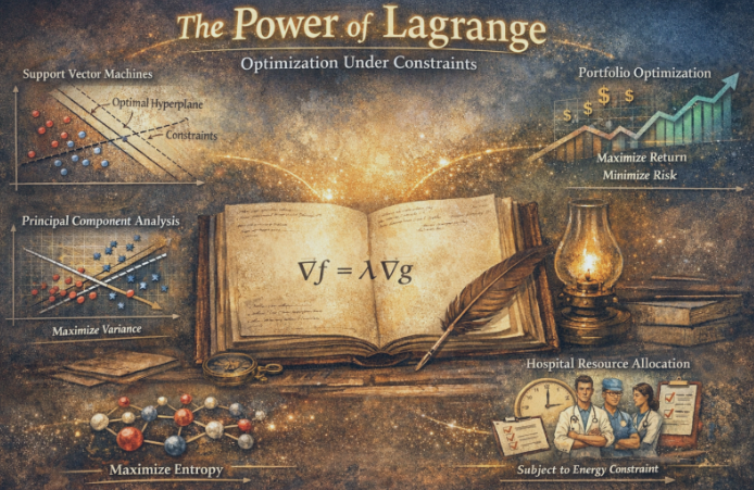
Lagrange’s work has influenced countless areas of science and engineering, but in this post, I want to focus specifically on optimization under constraints. It’s almost unbelievable how many modern fields depend on this idea.

Take support vector machines (SVMs), for example. Training an SVM involves finding the optimal separating hyperplane between classes while satisfying classification constraints. This is formulated as a constrained optimization problem, and the solution relies directly on Lagrange multipliers and their associated dual formulation. Without this framework, the mathematical structure behind SVMs simply wouldn’t exist in the form we use today.

Another striking example is principal component analysis (PCA). At its core, PCA can be derived as a constrained optimization problem: we maximize variance subject to a normalization constraint (typically that the principal direction has unit length). The solution emerges naturally using Lagrange multipliers, leading directly to an eigenvalue problem. What looks like linear algebra magic is, in fact, constrained optimization at work.

Resource allocation provides an even more tangible example. Consider hospital scheduling: how do you allocate doctors to meet patient demand while respecting constraints such as maximum working hours, medical specializations, patient health conditions, and labor regulations? These problems are formulated as constrained optimization models. The mathematical backbone of such systems descends directly from Lagrange’s framework.

Finance is another major beneficiary. Modern portfolio theory, for instance, involves maximizing expected return subject to a risk constraint (or minimizing risk for a target return). This is again a constrained optimization problem solved using Lagrangian methods.

Thermodynamics, statistics, engineering design, machine learning, operations research — all of these fields rely on structured optimization under constraints.

What began as an 18th-century mathematical insight became one of the most powerful ideas behind optimization and modern applications. Without further due, let’s get into it.

I want to start with a beautiful example inspired by Anil Ananthaswamy in his excellent book Why Machines Learn. If you haven’t read it, I highly recommend it. I’ll modify the example slightly, but the spirit remains the same.

Imagine you’re standing on the side of a valley, slowly walking downhill. Beneath the surface, hidden underground, there is a circular vein of an extremely valuable mineral. If you reach it first, you become rich. Others know about it too and the race to get to the mineral just starts.

You have two options:

1. Walk all the way down to the bottom of the valley and drill horizontally. This path is long and inefficient.
2. Descend the slope while positioning yourself exactly above the buried circular vein — meaning that if you dropped a vertical line from your feet straight down, it would intersect the center of the vein. From there, you drill straight down and reach it faster.

So, what’s the smartest move?

You are constrained to move along the surface of the hill. You cannot jump through the air. You cannot teleport underground. You can only move along the slope.

But you want to minimize the drilling distance.

This is exactly the structure of a constrained optimization problem.

• Objective: minimize the drilling distance.
• Constraint: the geometry of the hill — the surface you’re forced to walk on.

This is where Lagrange’s work comes into play. You want to find the minimum point on the surface you’re walking on, given the constraint that you must remain above the circular vein. Let’s visualize this in a Python notebook. I’ve prepared some code so you can see and understand what I’m talking about.

Main Surface (Valley)

The valley can be represented by the equation:

• f(x,y) = x² + 2y²

import numpy as np
import matplotlib.pyplot as plt
from mpl_toolkits.mplot3d import Axes3D

# Define the valley function
def f(x, y):
    return x**2 + 2*y**2

# Create grid
x = np.linspace(-3, 3, 400)
y = np.linspace(-3, 3, 400)
X, Y = np.meshgrid(x, y)
Z = f(X, Y)

# Create 3D plot
fig = plt.figure()
ax = fig.add_subplot(111, projection='3d')

ax.plot_surface(X, Y, Z)

ax.set_xlabel('X')
ax.set_ylabel('Y')
ax.set_zlabel('Z')

plt.show()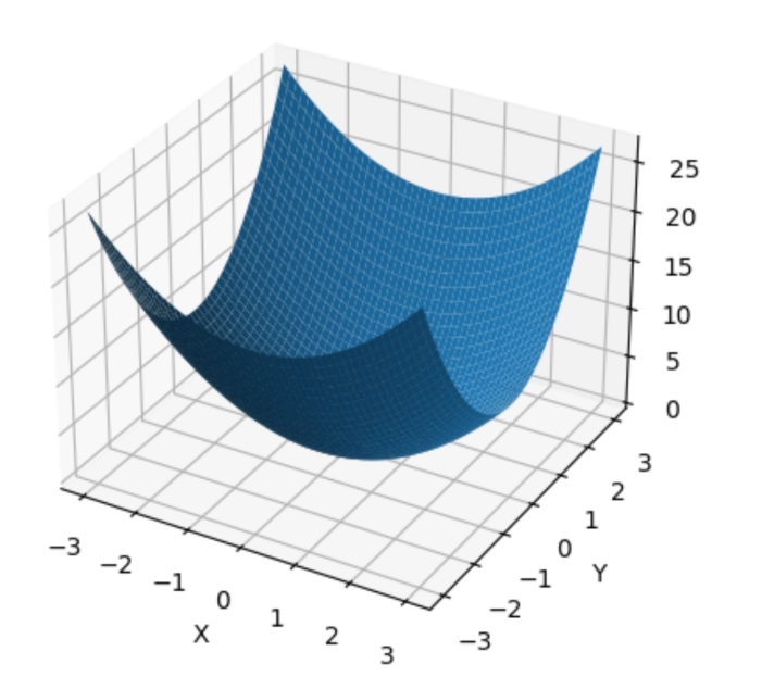

Constraint (Circular Vein)

The circular vein can be represented by the equation:

• x² + y² = 4

Let’s plot both the valley and the circular vein:

import numpy as np
import matplotlib.pyplot as plt
from mpl_toolkits.mplot3d import Axes3D

# Define the valley function
def f(x, y):
    return x**2 + 2*y**2

# Create grid
x = np.linspace(-3, 3, 400)
y = np.linspace(-3, 3, 400)
X, Y = np.meshgrid(x, y)
Z = f(X, Y)

# Create 3D plot
fig = plt.figure()
ax = fig.add_subplot(111, projection='3d')

# Plot valley surface
ax.plot_surface(X, Y, Z, alpha=0.3)

# Constraint: x^2 + y^2 = 4 (on z = 0 plane)
theta = np.linspace(0, 2*np.pi, 400)
x_c = 2 * np.cos(theta)
y_c = 2 * np.sin(theta)
z_c = np.zeros_like(theta)   # keep it flat in 2D

# Plot 2D constraint inside 3D space
ax.plot(x_c, y_c, z_c)

ax.set_xlabel('X')
ax.set_ylabel('Y')
ax.set_zlabel('Z')

plt.show()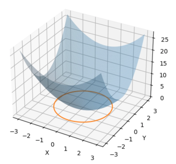

You can see the circular vein underground (orange curve).

Contour Lines

Contour lines (or level curves) are fundamental for our analysis. They are curves along which a function has a constant value. To visualize: all points at the same height from the bottom belong to the same contour line — just like a topographic map.

Back to our valley: if you stop at any point and draw a circle around the valley at the same height, that circle represents a contour line. Moving along it keeps you at the same height — you won’t descend further.

Contour lines are extremely useful because we can represent them in a 2D chart:

import numpy as np
import matplotlib.pyplot as plt
from mpl_toolkits.mplot3d import Axes3D

# Function
def f(x, y):
    return x**2 + 2*y**2

# Grid
x = np.linspace(-3, 3, 400)
y = np.linspace(-3, 3, 400)
X, Y = np.meshgrid(x, y)
Z = f(X, Y)

# Constraint circle
theta = np.linspace(0, 2*np.pi, 400)
x_c = 2 * np.cos(theta)
y_c = 2 * np.sin(theta)
z_c = np.zeros_like(theta)

# Create figure
fig = plt.figure(figsize=(12,5))

# 3D plot
ax = fig.add_subplot(121, projection='3d')

ax.plot_surface(X, Y, Z, alpha=0.3)

# Dashed constraint in z=0 plane
ax.plot(x_c, y_c, z_c, linestyle='--', color='black')

# Contour projection onto z=0
ax.contour(X, Y, Z, zdir='z', offset=0)

ax.set_xlabel('X')
ax.set_ylabel('Y')
ax.set_zlabel('Z')

# 2D contour plot
ax2 = fig.add_subplot(122)

ax2.contour(X, Y, Z)

# Dashed constraint circle
ax2.plot(x_c, y_c, linestyle='--', color='black')

ax2.set_aspect('equal', 'box')
ax2.set_xlabel('X')
ax2.set_ylabel('Y')

plt.show()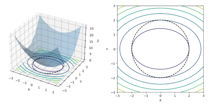

This graph may seem complex at first, but here’s the key:

• The dashed line represents the circular vein in both graphs.
• The other lines are contour lines of the valley.
• Darker lines indicate lower heights, lighter lines indicate higher points.

By combining contour lines and constraints, we can visually and mathematically understand where the optimal point lies — this is the heart of Lagrange multipliers.

The Aha Moment

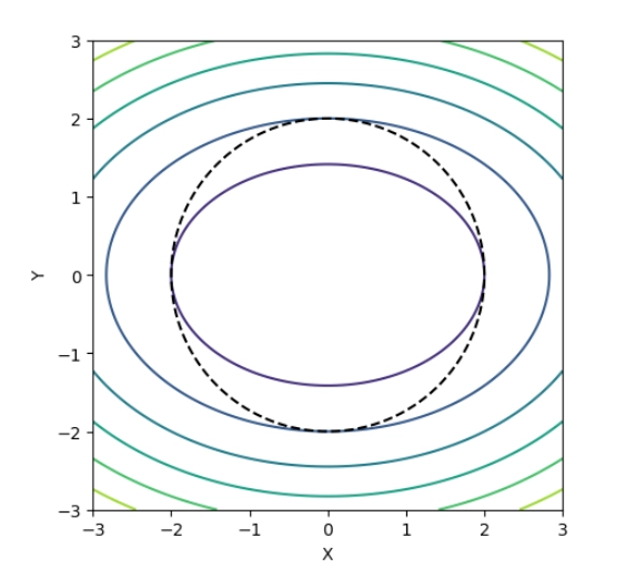
And here’s the beauty of it: once you overlay the contour lines of the valley with the circular constraint, it becomes instantly clear where the optimal point lies.

You don’t have to guess, you don’t have to wander around the valley. The solution is exactly where the contour line “just touches” the constraint. At this point, moving along the surface would no longer reduce your drilling distance — you’ve found the sweet spot.

If you check the next graph, you can see the contour line(the dark purple) is touching the mineral vein(dashed line) at -2 and 2 in the X axis and at -2 and 2 in Y axis. In other words, the contact points are (2,0),(−2,0) and (0,2),(0,−2).

Lagrange realized something remarkable: at the points where the constraint curve and a level curve of the function touch, the gradient of the function and the gradient of the constraint are parallel — they point in the same direction. Let’s check with the following code!

import numpy as np
import matplotlib.pyplot as plt

# Function
def f(x, y):
    return x**2 + 2*y**2

# Gradient
def grad_f(x, y):
    return np.array([2*x, 4*y])

# Grid
x = np.linspace(-3, 3, 400)
y = np.linspace(-3, 3, 400)
X, Y = np.meshgrid(x, y)
Z = f(X, Y)

# Constraint circle
theta = np.linspace(0, 2*np.pi, 400)
x_c = 2 * np.cos(theta)
y_c = 2 * np.sin(theta)

# Critical points
points = [(2,0), (-2,0), (0,2), (0,-2)]

# Plot
plt.figure(figsize=(6,6))

# Contours
plt.contour(X, Y, Z)

# Dashed constraint
plt.plot(x_c, y_c, linestyle='--', color='black')

# Plot gradients at critical points
for (x0, y0) in points:
    g = grad_f(x0, y0)
    plt.quiver(x0, y0, g[0], g[1], 
               angles='xy', scale_units='xy', scale=8)

    plt.scatter(x0, y0)

plt.gca().set_aspect('equal', 'box')
plt.xlabel('X')
plt.ylabel('Y')
plt.title("Contour + Constraint + Gradients")

plt.show()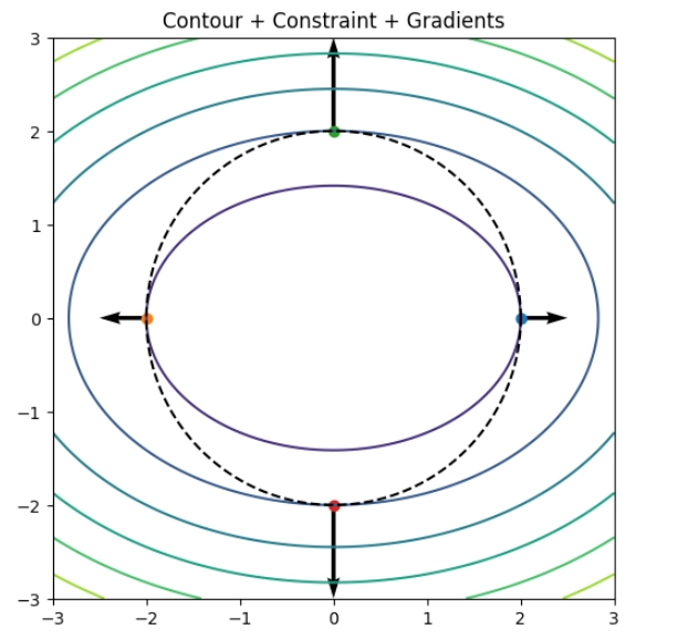

The gradient of the surface — the direction of steepest ascent — is parallel to the gradient of the constraint at the optimal point. When this happens, there is no way to move along the constraint that increases or decreases the function any further. In other words, you have reached a maximum or a minimum.

Lagrange formalized this insight in the powerful formula:

∇f(x,y)=λ∇g(x,y)

Here, the left-hand side is the gradient of the function we want to optimize, and the right-hand side is the gradient of the constraint.

The symbol λ (lambda) is a scalar multiplier — it tells us that the two vectors point in the same direction, even if their magnitudes are different. This mighty formula is known as the Lagrange multipliers and you can use it to get to the same conclusion we just got from a graphical point of view, it is a nice exercise!

Conclusion

What I love most about Lagrange multipliers isn’t the algebra. It’s the leap of insight that led Lagrange there in the first place. The equation is beautiful, but the idea behind it is even better. It’s kind of wild to think about how many real-world applications are powered by this one simple insight — I only scratched the surface at the start of this post.

Looking back, I wish I’d slowed down more in university and taken a moment to appreciate the elegance behind ideas like this. Some of the most powerful equations come from surprisingly simple ways of seeing the world.

Anyway, I hope you enjoyed reading this as much as I enjoyed writing it.