QuintNet — A 3D distributed Training Library

Ever wondered how companies train GPT-4, Llama, or Claude across thousands of GPUs?

The answer is 3D Parallelism — a combination of Data, Pipeline, and Tensor Parallelism that lets you train models too large for any single GPU. But most tutorials just show you how to use libraries like Megatron or DeepSpeed. They don’t explain how these systems actually work.

I built QuintNet to change that.

QuintNet is an educational PyTorch framework that implements 3D parallelism from first principles. No magic wrappers, no hidden complexity — just clean, documented Python code that shows you exactly how:

• Device Meshes organize GPUs into N-dimensional grids
• Process Groups enable efficient collective communication
• The 1F1B Schedule reduces memory usage by 50% during pipeline training
• Gradient Bucketing overlaps communication with computation

I trained a Vision Transformer on MNIST across 8 GPUs (2×2×2 mesh) and achieved 93.24% accuracy — proving the implementation actually works, not just in theory.

Here is my Github Repo — https://github.com/Wodlfvllf/QuintNet. Please Star If you find it helpful.

Table of Contents

1. Overview: What is 3D Parallelism?
2. The Device Mesh
3. Model Wrapping Pipeline
4. Data Flow Architecture
5. Pipeline Parallelism Deep Dive
6. The 1F1B Schedule
7. Gradient Synchronization
8. Complete Training Loop

1. Overview: What is 3D Parallelism?

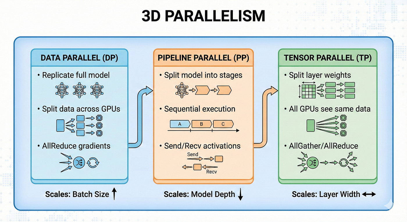
A conceptual diagram outlining the three components of 3D parallelism (Data, Pipeline, and Tensor Parallelism), how they split the workload, their communication methods, and what they scale.

Training large deep learning models requires more memory and compute than a single GPU can provide. 3D Parallelism is the solution: it combines three complementary strategies to distribute the workload across many GPUs.

The Three Dimensions

Data Parallelism (DP) is the most intuitive approach. Imagine you have a book to read, and you want to finish faster. If you have 4 friends, you can photocopy the book 4 times, give each friend a copy, and have each person read different chapters. At the end, you all share what you learned. In deep learning terms:

• Every GPU gets a complete copy of the model
• Each GPU processes a different batch of training data
• After computing gradients, all GPUs synchronize by averaging their gradients
• This scales the effective batch size linearly with the number of GPUs

Pipeline Parallelism (PP) takes a different approach. Instead of copying the entire book, you split it into chapters. Friend 1 reads chapter 1, then passes the summary to Friend 2 who reads chapter 2, and so on. In deep learning:

• The model is split into sequential stages (e.g., first half of layers on GPU 0, second half on GPU 1)
• Data flows through the pipeline like an assembly line
• Each GPU only holds a portion of the model, reducing memory requirements
• This is essential when a single model is too large to fit on one GPU

Tensor Parallelism (TP) goes even deeper. What if a single chapter is too long for one person? You split each page in half — Person A reads the left column, Person B reads the right column, and they combine their understanding. In deep learning:

• Individual layer weights are sharded across GPUs
• Each GPU computes a portion of the output for each layer
• Results are combined using collective communication
• This is crucial for very wide layers (like the FFN layers in LLMs with thousands of hidden dimensions)

When to Use Each:

The beauty of 3D parallelism is that each strategy is orthogonal — they scale different dimensions of the training workload:

2. The Device Mesh

Before we can train in 3D, we need to organize our GPUs into a logical structure. The Device Mesh is an N-dimensional grid that maps physical GPUs to their roles in each parallelism dimension.

Understanding the Mesh

Think of the device mesh as a 3D coordinate system. Each GPU has a unique address like (dp_rank, tp_rank, pp_rank). For our configuration with 8 GPUs and mesh dimensions [2, 2, 2]:

• DP dimension: 2 replicas of the model
• TP dimension: Each layer split across 2 GPUs
• PP dimension: Model split into 2 pipeline stages

This creates a logical cube where each corner represents a GPU with specific responsibilities.

Process Groups Created — Who Talks to Whom?

GPUs don’t communicate randomly — they form process groups based on their roles:

Data Parallel Groups connect GPUs that have the same model shard but process different data. After computing gradients, these GPUs must synchronize. In our mesh:

• Group 0: GPU 0 ↔ GPU 4 (both have PP stage 0, TP shard 0)
• Group 1: GPU 1 ↔ GPU 5 (both have PP stage 1, TP shard 0)

These groups perform AllReduce operations to average gradients.

Pipeline Parallel Groups connect GPUs that form a single pipeline. Data flows sequentially through these GPUs:

• Group 0: GPU 0 → GPU 1 (stages 0 and 1 for one DP+TP replica)
• Group 1: GPU 4 → GPU 5 (stages 0 and 1 for another replica)

These groups use point-to-point Send/Recv operations to pass activations.

Tensor Parallel Groups connect GPUs that jointly compute each layer:

• Group 0: GPU 0 ↔ GPU 2 (same DP rank, same PP stage)
• Group 1: GPU 1 ↔ GPU 3

These groups use AllGather and AllReduce to combine partial results.

Why Process Groups Matter

Efficient distributed training depends on minimizing communication overhead. By organizing GPUs into groups:

1. Reduced communication scope: AllReduce across 2 GPUs is faster than across 8
2. Parallel communication: Different groups can communicate simultaneously
3. Optimal placement: GPUs in the same group should be on the same node when possible

# Data Parallel groups (GPUs that sync gradients)
DP Group 0: [GPU 0, GPU 4]  # Same TP rank, same PP stage
DP Group 1: [GPU 1, GPU 5]
DP Group 2: [GPU 2, GPU 6]
DP Group 3: [GPU 3, GPU 7]

# Pipeline Parallel groups (GPUs that pass activations)
PP Group 0: [GPU 0, GPU 1]  # Same DP rank, same TP rank
PP Group 1: [GPU 2, GPU 3]
PP Group 2: [GPU 4, GPU 5]
PP Group 3: [GPU 6, GPU 7]

# Tensor Parallel groups (GPUs that shard layers)
TP Group 0: [GPU 0, GPU 2]  # Same DP rank, same PP stage
TP Group 1: [GPU 1, GPU 3]
TP Group 2: [GPU 4, GPU 6]
TP Group 3: [GPU 5, GPU 7]

3. Model Wrapping Pipeline

Transforming a regular PyTorch model into a 3D parallel model requires a series of wrapping transformations. Each wrapper adds one dimension of parallelism, and the order matters.

Step 1: Tensor Parallelism (Innermost)

First, we apply Tensor Parallelism to shard individual layers. This is the innermost transformation because it modifies the model’s computational graph at the finest granularity.

For each nn.Linear layer, we decide whether to use Column Parallelism or Row Parallelism:

Column Parallel Linear splits the weight matrix along the output dimension. If a layer projects from 768 → 3072 dimensions with TP=2:

• GPU 0 holds weights of shape [768, 1536] (first half of outputs)
• GPU 1 holds weights of shape [768, 1536] (second half of outputs)

During forward pass, each GPU computes half the output, then they AllGather to reconstruct the full output. The key insight is that both GPUs receive the full input but produce complementary outputs.

Row Parallel Linear splits along the input dimension. If a layer projects from 3072 → 768 with TP=2:

• GPU 0 holds weights of shape [1536, 768] (processes first half of inputs)
• GPU 1 holds weights of shape [1536, 768] (processes second half of inputs)

During forward pass, each GPU computes a partial result, then they AllReduce to combine them. Here, each GPU receives half the input and must coordinate to produce the final output.

In transformer architectures, we typically alternate: the attention projection uses Column Parallel, and the output projection uses Row Parallel. This minimizes communication by exploiting the natural data flow.

Step 2: Pipeline Parallelism (Middle)

After tensor parallelism is applied within layers, we split the model into sequential stages for pipeline parallelism.

The key challenge is where to split. We need:

• Roughly equal compute per stage (for load balancing)
• Clear boundaries between stages (for clean activation tensors)
• Minimal cross-stage communication

For a transformer with 8 blocks split across 2 stages:

• Stage 0: Embedding layer + Blocks 0–3
• Stage 1: Blocks 4–7 + Classification head

Only the intermediate activations (hidden states between stages) need to be communicated. For a ViT, this is a tensor of shape [batch, sequence_length, hidden_dim].

Step 3: Data Parallelism (Outermost)

Finally, we wrap the entire pipeline-and-tensor-parallel model with Data Parallelism.

This wrapper:

1. Registers gradient hooks on all parameters
2. Groups parameters into buckets for efficient communication
3. Performs AllReduce after the backward pass

The key insight is that DP wraps the entire distributed model. Each DP replica contains a complete pipeline with all TP shards for its portion.

The Complete Wrapping Chain

The final model structure is:

Detailed Transformation:

# STEP 1: Original Model
model = VisionTransformer(
    embedding=PatchEmbedding(),
    blocks=[TransformerBlock() for _ in range(8)],
    head=ClassificationHead()
)

# STEP 2: Tensor Parallel - Shard Linear layers
# Each nn.Linear becomes ColumnParallelLinear or RowParallelLinear
# Weight matrix is split across TP group

# Before: Linear(in=768, out=3072)
# After on GPU 0: ColumnParallelLinear(in=768, out=1536)  # First half
# After on GPU 2: ColumnParallelLinear(in=768, out=1536)  # Second half

# STEP 3: Pipeline Parallel - Split into stages
# Model is partitioned across PP stages

# GPU (pp=0): embedding + blocks[0:4]
# GPU (pp=1): blocks[4:8] + head

# STEP 4: Data Parallel - Add gradient sync
# Wraps model with gradient reduction hooks
# After backward, AllReduce across DP group

4. Data Flow Architecture

Understanding how data flows through the 3D mesh is crucial for debugging and optimization.

The Journey of a Batch

Let’s trace a single training batch through the system:

1. Data Loading and Distribution

The DistributedSampler ensures each DP replica sees different data. With 60,000 MNIST images and DP=2:

• DP replica 0 sees 30,000 images (indices 0, 2, 4, …)
• DP replica 1 sees 30,000 images (indices 1, 3, 5, …)

Importantly, all GPUs within a DP replica see the same batch. The PP and TP dimensions don’t affect data distribution — only the DP dimension does.

2. First Pipeline Stage (Forward)

The batch arrives at Stage 0 GPUs. If TP=2:

• GPU 0 and GPU 2 both receive the same input tensor
• Each applies their portion of tensor-parallel layers
• They coordinate via AllGather/AllReduce within TP groups

After processing, Stage 0 produces an activation tensor representing the intermediate hidden state.

3. Activation Transfer

The activation tensor is sent from Stage 0 to Stage 1:

• GPU 0 sends to GPU 1 (within the same pipeline)
• GPU 2 sends to GPU 3 (within the same pipeline)

This uses point-to-point NCCL Send and Recv operations. The receiving GPU blocks until the tensor arrives.

4. Subsequent Stages

Stage 1 GPUs receive the activation and continue the forward pass. They:

• Process through their allocated layers
• Apply tensor parallelism within their TP group
• Compute the final output (logits for classification)

5. Loss Computation

Only the last pipeline stage computes the loss. This is crucial because:

• Only the last stage has the final model output
• The loss scalar becomes the “input gradient” for backward pass
• Metrics (accuracy) are only meaningful on the last stage

6. Backward Pass

Gradients flow in reverse:

• Last stage computes gradients for its parameters
• Gradient of activations is sent back to previous stages
• Each stage computes its parameter gradients

7. Gradient Synchronization

After backward pass completes on all stages:

• Each parameter’s gradient is reduced across DP replicas
• This uses AllReduce within DP groups
• After sync, all DP replicas have identical averaged gradients

8. Optimizer Step

All GPUs update their parameters simultaneously. Since gradients are synchronized, all DP replicas maintain identical weights.

Key Insight:

• DP dimension: Different data, same model computation
• PP dimension: Same data flows sequentially through stages
• TP dimension: Same data, computation is split within each layer

5. Pipeline Parallelism Deep Dive

Pipeline Parallelism is the most complex dimension because it introduces temporal dependencies — stages must coordinate their execution order.

The Bubble Problem

Consider a naive approach: run all forward passes, then all backward passes. With 4 stages:

Time →
Stage 0: FFFF........BBBB
Stage 1: .FFFF......BBBB.
Stage 2: ..FFFF....BBBB..
Stage 3: ...FFFF..BBBB...

The dots represent idle time (the “bubble”). GPUs wait for:

• Forward: Previous stage to produce activations
• Backward: Next stage to produce gradients

The bubble can be 50% or more of total training time. This is unacceptable for efficiency.

Micro-batching to the Rescue

The solution is micro-batching: split each batch into smaller pieces and pipeline them. With 8 micro-batches:

Stage 0: F0 F1 F2 F3 F4 F5 F6 F7 . . . . B0 B1 B2 B3 B4 B5 B6 B7
Stage 1: . F0 F1 F2 F3 F4 F5 F6 F7 . . . . B0 B1 B2 B3 B4 B5 B6 B7

Now Stage 0 can work on F1 while Stage 1 works on F0. The pipeline stays more utilized.

But there’s still a problem: memory. If we run all 8 forwards before any backward, we must store 8 sets of activations per stage. For large models, this can exceed GPU memory.

Enter 1F1B

The One Forward, One Backward (1F1B) schedule solves this elegantly, as we’ll explore in the next section.

Stage Assignment

How do we decide which layers go to which stage? The algorithm:

1. List all “blocks” (transformer blocks, embedding, head)
2. Count parameters and estimate compute per block
3. Assign blocks to stages to balance workload
4. Keep sequential blocks together when possible

For QuintNet with 8 transformer blocks and 2 stages:

• Stage 0: Embedding + Blocks 0–3 (first half)
• Stage 1: Blocks 4–7 + Classification Head (second half)

Communication Pattern:

6. The 1F1B Schedule

The 1F1B (One Forward, One Backward) schedule is a carefully choreographed dance that maximizes GPU utilization while minimizing memory usage.

The Three Phases

Warmup Phase: Fill the pipeline with forward passes.

At the start, later stages have no activations to process. We run enough forwards to “prime” the pipeline:

• Stage 0 runs forward for micro-batches 0, 1, 2, 3
• Each forward’s output is sent to the next stage
• By the time Stage 3 finishes its first forward, the pipeline is “full”

The number of warmup steps equals min(num_stages - stage_rank - 1, total_microbatches).

Steady State Phase: Alternate 1 Forward, 1 Backward.

This is the magic of 1F1B. Each stage alternates between:

1. Complete one forward pass (for the next micro-batch)
2. Complete one backward pass (for an earlier micro-batch)

Why does this work? The key insight: activations from micro-batch K are only needed for backward pass of micro-batch K. By interleaving, we can process the backward for K while doing forward for K+1.

Memory analysis:

• At any time, each stage holds activations for at most ~num_stages micro-batches
• Compare to naive: would hold all micro-batch activations
• For 4 stages, 8 micro-batches: 4 activations vs 8 (50% reduction!)

Cooldown Phase: Drain remaining backward passes.

After all forwards complete, we still have backward passes in flight. We run these to completion, draining the pipeline.

Why 1F1B is Essential for Large Models

Consider training a 10B parameter model with activation memory of 2GB per micro-batch:

ScheduleMicro-batchesPeak Activation MemoryNaive (all F then B)816 GB1F1B88 GB (4 stages)

This 50% reduction can mean the difference between fitting in GPU memory or not.

Communication Overlap

An advanced optimization: overlap communication with computation. While GPU computes forward for micro-batch K, it can simultaneously receive activations for micro-batch K+1. QuintNet uses PyTorch’s async operations for this:

recv_handle = dist.irecv(tensor, src=prev_stage)
compute_forward(...)  # Overlapped execution
recv_handle.wait()

7. Gradient Synchronization

After backward passes complete, gradients must be synchronized across DP replicas to maintain model consistency.

The Challenge

Each DP replica computes gradients based on different data:

• Replica 0: Gradients from images 0, 2, 4, …
• Replica 1: Gradients from images 1, 3, 5, …

For correct optimization, we need the average gradient across all data. This is mathematically equivalent to training on the full batch.

AllReduce Operation

AllReduce is the workhorse of gradient synchronization. It:

1. Takes a tensor from each GPU in the group
2. Computes an element-wise reduction (sum or average)
3. Returns the result to all GPUs

After AllReduce, every GPU in the DP group has identical gradients:

gradient_0 = gradient_1 = (original_0 + original_1) / 2

Gradient Bucketing

Calling AllReduce for each parameter individually is inefficient. The overhead of initiating communication dominates for small tensors.

Bucketing groups parameters into larger chunks (default: 25MB):

1. As gradients are computed, they’re added to a bucket
2. When a bucket is full, AllReduce is triggered
3. Multiple small AllReduces become fewer large ones

This exploits the fact that bandwidth is limited, but so is latency. Larger transfers amortize the fixed overhead of each communication.

Gradient Computation Order

PyTorch computes gradients in reverse order of the forward pass. We register gradient hooks that:

1. Copy gradient to the appropriate bucket
2. Mark the parameter as “ready”
3. When all parameters in a bucket are ready, trigger AllReduce

This allows overlapping gradient computation with communication. While GPU computes gradients for earlier layers, it can simultaneously sync later layers’ gradients.

Handling Pipeline + Data Parallelism

With both PP and DP, synchronization becomes nuanced:

1. Each pipeline stage has its own parameters
2. DP sync only happens within each stage
3. Parameters on different stages sync with different DP groups

This is why process groups are carefully constructed — each parameter knows exactly which GPUs it should sync with.

8. Complete Training Loop

The full training loop with all components:

Summary: The Big Picture