Decoding 4D Gaussian Splatting: A Journey into Real-Time Dynamic Scene Rendering

How factorizing space and time unlocks 80+ FPS for complex 4D environments.

Read Time: 8–10 minutes

Rendering static 3D scenes in real-time was a massive breakthrough. But the real world isn’t static. People move, liquids pour, and objects deform. Extending 3D-GS to dynamic scenes (4D) seems conceptually straightforward just track the points over time but practically, it introduces a massive memory bottleneck.

Recently, I dove deep into the architecture of 4D Gaussian Splatting (4D-GS). Through a series of mathematical breakdowns and architectural explorations, a remarkably elegant solution emerged. Here is the story of how 4D-GS bypasses the memory explosion of dynamic rendering by replacing brute-force tracking with a highly optimized, factorized deformation field.

The Memory Bottleneck: Why Vanilla Tracking Fails

To understand the genius of 4D-GS, we first have to understand the problem it solves.

In traditional dynamic NeRFs, the network maps an 8D input space (x, d, t, λ) to color and density, where λ is a latent code used to handle complex topological changes like surfaces splitting or merging. While effective, the implicit nature of NeRFs inherently throttles rendering speeds.

3D Gaussian Splatting solves the speed issue by explicitly representing the scene as millions of point-like Gaussians that can be rapidly rasterized. However, if you attempt to make this dynamic by storing the position, rotation, and scaling of every single Gaussian for every single frame (100 million Gaussians x 100 frames), your VRAM requirements scale linearly into oblivion.

The breakthrough of 4D-GS is that it completely Abandons the idea of storing per-frame Gaussians. Instead, it maintains only one canonical set of 3D Gaussians. It then uses a lightweight neural network to act as a deformation field, calculating exactly how those base Gaussians need to shift, stretch, and rotate for any given timestamp.

The rendering equation elegantly simplifies to:

G’ = G + ΔG

Where the deformed scene (G’) is simply the static baseline (G) plus the neural-predicted change (ΔG).

Deconstructing the Deformation Field

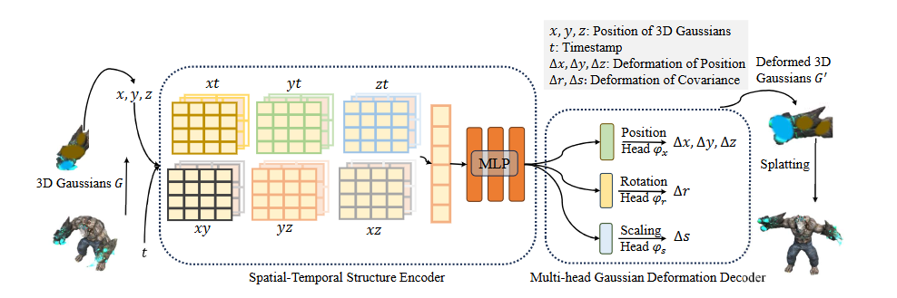
How do we actually compute ΔG without blowing up our memory? The 4D-GS architecture splits this task into two distinct phases: The Observer (Encoder) and The Director (Decoder).

1. The Spatial-Temporal Structure Encoder (The Observer)

If we want to deform a point, we need to understand its context. Where is it? What time is it? What are its neighbors doing?

The naive approach would be to map the scene into a massive 4D neural voxel grid (x, y, z, t). But as established, O(N⁴) memory scaling is a non-starter. Instead, 4D-GS borrows a brilliant technique from models like HexPlane and K-Planes: decomposition.

The massive 4D space is flattened into 6 lightweight, multi-resolution 2D planes:

• Spatial Planes: XY, XZ, YZ
• Temporal Planes: XT, YT, ZT

When the network queries a continuous Gaussian coordinate like μ = (1.234, 5.678, 2.0) at time t, it doesn’t land perfectly on the discrete grid vertices of these planes. The encoder uses bilinear interpolation to check the four nearest grid corners on each plane, calculates a distance-weighted average, and extracts 6 specific feature vectors.

These 6 vectors are mathematically bound together via an element-wise (Hadamard) product:

This single, dense vector (f_h) is then passed through a tiny Multi-Layer Perceptron (MLP) to create our final, compressed context vector: f_d.

The Nitty-Gritty: Initializing the HexPlanes

A neural network’s success often hinges on its starting state. In 4D-GS, the initialization of the six feature planes is a masterclass in mathematical intuition. Before the first forward pass, the explicit feature grids must be populated. The spatial planes (XY, XZ, and YZ) are initialized with uniform random values in the range [0.1, 0.5]. This provides enough variation for the network to begin learning meaningful spatial features from the very start. The spatio-temporal planes (XT, YT, and ZT), however, are initialized to exactly 1.

Why initialize temporal features to 1?

The answer lies in the feature aggregation step, where features from different planes are combined using element-wise multiplication. If the temporal features are initialized to 1, multiplying them with the spatial features produces no change: x × 1 = x

As a result, the model initially behaves as if the entire world is static. This is a deliberate design choice. Rather than assuming motion exists everywhere, the network starts with a static scene and is forced to modify the spatio-temporal features only when the loss function indicates that motion is necessary to explain the observed data.

In other words, movement is not built into the model by default. It must be earned through optimization. This encourages the network to learn deformations only where genuine motion exists, leading to a more stable and physically meaningful representation of dynamic scenes.

2. The Multi-Head Decoder (The Director)

With the context gathered, the multi-head decoder translates the feature vector (fd) into physical instructions. Separate linear heads predict the exact physical residuals:

• Position Shift: ΔX
• Rotation Shift: Δr
• Scale Shift: Δs

These values are added to the canonical Gaussians, and the scene is handed off to the differentiable rasterizer for real-time tile-based splatting.

During my deep dive, I noticed a fascinating architectural constraint: the main 4D-GS pipeline does not predict changes for color ΔC or opacity Δα.

Why restrict the network? Because neural networks are notoriously lazy.

If given the ability to freely alter color and opacity, the network might cheat to simulate motion. Instead of mathematically dragging a Gaussian from Point A to Point B, it could simply drop the opacity of the point at A to zero, raise the opacity of a point at B to one, and flash their colors to fake a moving object.

This ruins the fundamental physical geometry of the scene and destroys any capability for downstream 3D tracking. By locking color and opacity, the authors force the network to learn the true physical deformation. (They do note, however, that predicting ΔC and Δα can be reactivated for edge cases involving fluids or extreme non-rigid motions ).

Navigating the Loss Landscape: Training Dynamics

Training a dynamic field from scratch is chaotic. The optimizer has to figure out the base geometry and the motion simultaneously. To stabilize this, 4D-GS relies on a two-stage training paradigm:

1. The Static Warm-Up: For the first 3000 iterations, the deformation field is entirely disabled. The model acts as a vanilla 3D-GS model, forcing the canonical Gaussians to find their optimal static geometry.
2. The 4D Optimization: The deformation field is turned on. The network now predicts motion, renders the image via differential splatting, and computes the loss.

The objective function elegantly balances accuracy with smoothness:

The L1 loss forces the rendered output to match the ground truth Î. Crucially, the Total Variation Ltv loss is applied directly to the HexPlane grids. It penalizes erratic jumps between adjacent grid cells, mathematically enforcing smooth, continuous motion across the scene.

The Backward Pass: A Tale of Two Paths

Because the splatting function S is differentiable, the total loss L can be backpropagated through the entire pipeline using the chain rule.

During the backward pass, the optimizer calculates the gradients of the loss with respect to all learnable parameters. These gradients fork into two distinct paths:

Path A: Updating the Canonical Gaussians (G)

The gradients flow all the way back to the base canonical point cloud to update the starting positions and properties. The gradient dL/dG updates the base geometry, ensuring the canonical shape remains accurate.

Path B: Updating the Deformation Field (F)

The gradients flow through the addition operation:

G’ = G + ΔG

and into the neural network to adjust how it predicts motion.

Here, the network applies highly specific learning-rate schedules to ensure stability:

The Decoder Weights (θD): The gradient dL/dθD updates the weights of the multi-head MLP. The paper notes that this decoder is trained conservatively, with a learning rate that decays from 1.6 × 10⁻⁴ down to 1.6 × 10⁻⁵.

The HexPlane Features (Rl): The gradient dL/dRl updates the actual feature values stored inside the six multi-resolution HexPlanes. Because these are explicit grid parameters rather than deep network weights, they learn slightly faster, with a learning rate decaying from 1.6 × 10⁻³ down to 1.6 × 10⁻⁴.

By running this optimization loop for up to 20,000 iterations, the canonical Gaussians settle into their optimal base shapes, while the HexPlanes and MLP gradually adjust their parameters until the predicted deformations accurately reproduce the dynamic motion present in the video.

Multi-View vs. Monocular Realities

The true test of any dynamic renderer is its data input. 4D-GS handles different camera setups with distinct advantages:

• Multi-View (e.g., Neu3D): With 15–20 cameras firing simultaneously, the network calculates the 4D deformation once per timestamp, but splats and calculates loss from 20 different angles. This dense feedback prevents the model from “flattening” geometry to cheat a single camera perspective.
• Monocular (e.g., D-NeRF): Given only one camera angle per timestamp, the network must rely heavily on the HexPlane’s temporal continuity to infer 3D motion.

While it excels in many scenarios, the architecture still faces open challenges. In datasets like HyperNeRF, where cameras physically move forward, the deformation field can fall into local minima — struggling to mathematically separate the motion of the camera from the motion of the subject. Furthermore, extreme, rapid motions without multi-view overlap remain a hurdle for the current encoder formulation.

Key Takeaways

The transition from static to dynamic point-cloud rendering is not just about adding a time variable; it requires a fundamental restructuring of how we store and query information.

• Deformation Over Tracking: By maintaining a single canonical set of Gaussians and predicting Deformations, memory scales with the complexity of the motion network, not the length of the video.
• Decomposition is King: Factorizing 4D space into six 2D planes allows for rapid feature querying via bilinear interpolation, completely bypassing the O(N⁴) memory curse of 4D voxels.
• Constrain to Train: Preventing the network from altering color and opacity forces it to learn genuine physical movement, enabling highly accurate 3D tracking alongside rendering.

4D-GS proves that with smart factorization and strategic constraints, explicit representations can conquer the temporal dimension without sacrificing the real-time performance that made them revolutionary in the first place.

References

Core Paper

1. Wu, G., Yi, T., Fang, J., Xie, L., Zhang, X., Wang, W., Liu, W., Tian, Q., and Wang, X. 4D Gaussian Splatting for Real-Time Dynamic Scene Rendering CVPR 2024. https://arxiv.org/abs/2310.08528

Foundational Gaussian Splatting Work

1. Kerbl, B., Kopanas, G., Leimkühler, T., and Drettakis, G. 3D Gaussian Splatting for Real-Time Radiance Field Rendering SIGGRAPH 2023. https://arxiv.org/abs/2308.04079

Factorized Plane Representations

1. Fridovich-Keil, S., Meanti, G., Warburg, F. R., Recht, B., and Kanazawa, A. K-Planes: Explicit Radiance Fields in Space, Time, and Appearance CVPR 2023. https://arxiv.org/abs/2301.10241
2. Cao, A., Johnson, J., and Ye, Y. HexPlane: A Fast Representation for Dynamic Scenes CVPR 2023. https://arxiv.org/abs/2301.09632