Deriving DDIM Reverse Sampling from First Principles, with a TensorFlow Implementation

A math-first walkthrough of DDPM/DDIM sampling, velocity prediction, and CIFAR-10 experiments in TensorFlow/Keras.

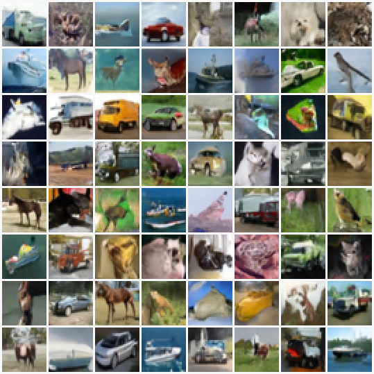
CIFAR-10 samples from the current best net01 split: cosine scheduler, noise prediction, min-SNR loss weighting, FID 16.507735

## Why I wrote this

Diffusion implementations are easy to run and surprisingly easy to misunderstand. A sampler can look correct at the API level while hiding small notation mismatches: whether alpha_t means per-step alpha or cumulative alpha, whether a model predicts noise or velocity, or whether a reverse step is adjacent DDPM or a skipped DDIM step.

This repository is my attempt to make the implementation follow the derivation directly. The full PDF derives the variance-preserving forward process, the DDPM posterior, and the DDIM reverse update. This Medium version is the short story: the identities I found most useful while building and testing the TensorFlow implementation.

Full repo:

https://github.com/supply1976/fast-ddim-tf

Full math note:

https://github.com/supply1976/fast-ddim-tf/blob/main/docs/math_note/Diffusion_Model_Mathematics_Notes.pdf

## The one equation that drives training

In the variance-preserving diffusion process, a clean image x_0 is mixed with Gaussian noise to produce a noisy image x_t:

Here alpha_t is the cumulative signal power. Some papers write this as alpha_bar_t; in my code and notes I use alpha_t for the cumulative quantity.

This direct formula is the reason diffusion training is efficient. We do not simulate every noising step during training. We sample a timestep t, sample Gaussian noise epsilon, construct x_t, and train the network to predict one of several equivalent targets.

## Three prediction targets

The implementation supports three targets:

1. Noise prediction: train the network to predict epsilon.

2. Image prediction: train the network to predict x_0.

3. Velocity prediction: train the network to predict a rotated coordinate v_t.

Noise prediction is the classic DDPM choice. If the model predicts noise, the clean-image estimate is:

x_0^theta = (x_t — sqrt(1 — alpha_t) epsilon_theta) / sqrt(alpha_t)

Image prediction reverses that relationship:

epsilon_theta = (x_t — sqrt(alpha_t) x_0^theta) / sqrt(1 — alpha_t)

Velocity prediction, used by Salimans and Ho in progressive distillation work, uses:

From a predicted velocity v_theta, the implementation converts back to clean-image and noise estimates:

x_0^theta = sqrt(alpha_t) x_t — sqrt(1 — alpha_t) v_theta

epsilon_theta = sqrt(alpha_t) v_theta + sqrt(1 — alpha_t) x_t

The benefit is numerical: velocity prediction keeps the target scale better balanced across noise levels.

## From DDPM posterior to DDIM sampling

The exact reverse process q(x_s | x_t) depends on the unknown data distribution, so we cannot write it directly. But the posterior conditioned on the original clean image is Gaussian:

q(x_s | x_t, x_0) = N(mu_{s,t}(x_t, x_0), Sigma_{s,t}² I)

DDPM sampling replaces the unknown x_0 with the model estimate x_0^theta, then adds Gaussian noise from the posterior variance.

DDIM rewrites the same ingredients in a form that exposes the predicted clean image and predicted noise:

The parameter eta controls stochasticity:

• eta = 0: deterministic DDIM sampling

• eta = 1: DDPM-equivalent posterior variance

• 0 < eta < 1: interpolation between the two

The useful part is that s and t do not need to be adjacent training timesteps. We can skip timesteps at sampling time and generate faster.

## Continuous derivation, discrete implementation

The full note derives the reverse step for arbitrary reverse time pairs (s, t) with s < t. That is the continuous-time viewpoint.

The current TensorFlow implementation uses a uniform reverse timestep grid controlled by REVERSE_STEPS. For example, a model trained with 1000 diffusion timesteps can sample with 100 DDIM reverse steps by selecting a descending uniform subset.

That distinction matters. The math supports arbitrary pairs; the current sampler chooses a uniform schedule for simplicity and reproducibility.

## References

• Jonathan Ho, Ajay Jain, and Pieter Abbeel. Denoising Diffusion Probabilistic Models. NeurIPS, 2020.

• Jiaming Song, Chenlin Meng, and Stefano Ermon. Denoising Diffusion Implicit Models. ICLR, 2021.

• Alex Nichol and Prafulla Dhariwal. Improved Denoising Diffusion Probabilistic Models. ICML, 2021.

• Tim Salimans and Jonathan Ho. Progressive Distillation for Fast Sampling of Diffusion Models. ICLR, 2022.

• Yang Song, Jascha Sohl-Dickstein, Diederik P. Kingma, Abhishek Kumar, Stefano Ermon, and Ben Poole. Score-Based Generative Modeling through Stochastic Differential Equations. ICLR, 2021.