Backpropagation through time — The RNN way

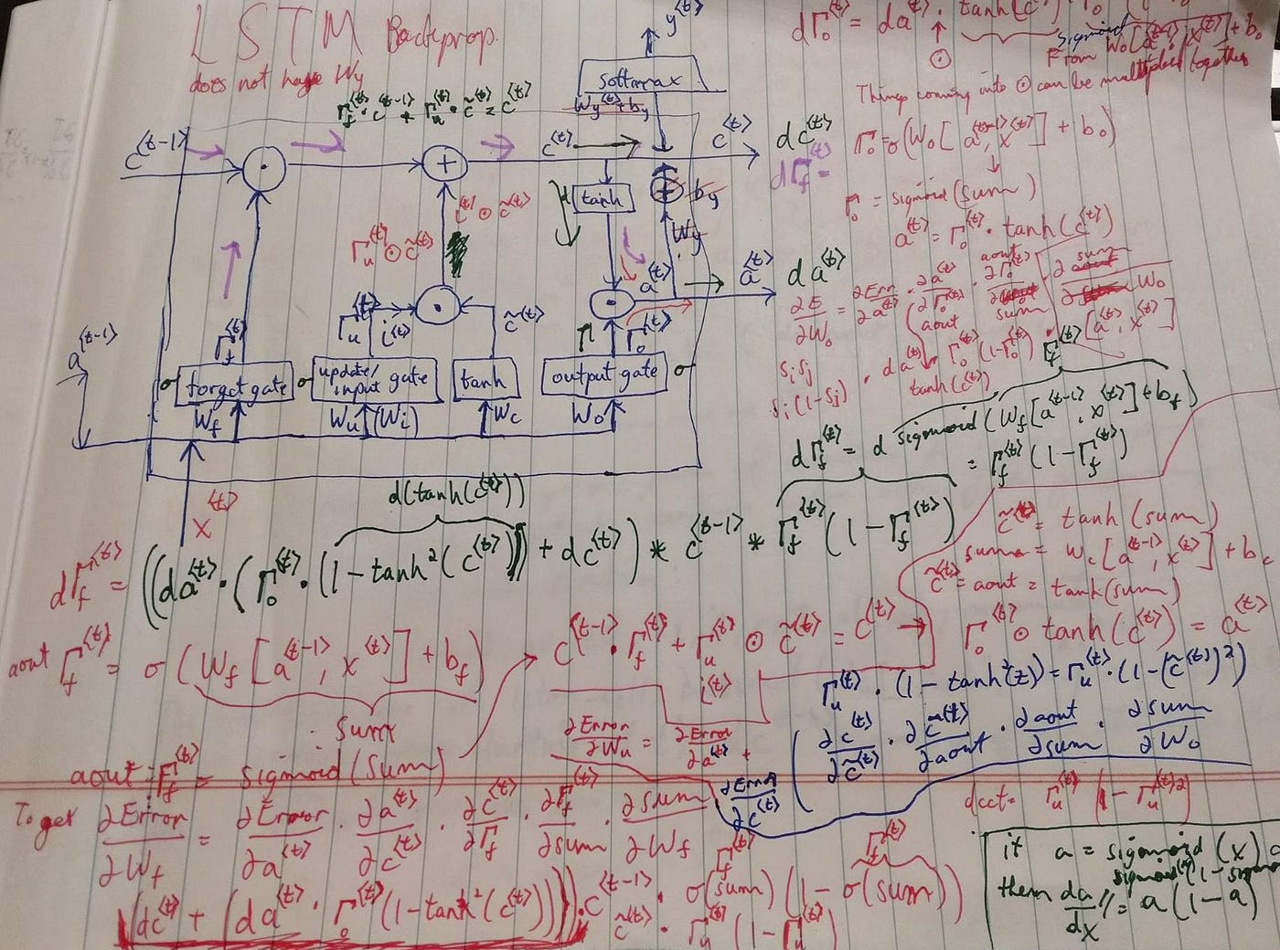
Source: KDNuggets

The motivation to capture temporal features through neural networks slowly emerged when neural networks were still under the hood. Such neural networks are commonly referred to as sequence learning models. One should know some basic artificial neural network structures: recurrent neural networks, long-short-term memory, and gated recurrent units. Although the above networks are not extensively used, understanding them makes it easier to learn other sequence models, like the family of autoencoders and other SOTAs.

It was difficult to train these models because:

• The recurrent function makes the feedforward process no more a simple feedforward
• Backpropagation through time (BPTT) takes “time” to register in our heads
• The vanishing and exploding gradients problem
• Training such models took more time

This article will provide an overview of BPTT and how it makes sequence models learn their objective functions. The caveat of BPTT is when the models have a long sequence of inputs which makes backpropagation inefficient because of the long chains. This is popularly known as the vanishing and exploding gradients problem. But LSTM and GRU tackle this by regulating the forward flow of inputs and the backward flow of the gradients using gates. They use BPTT, and they also learn to regulate information flow.

Tejas T A has written a beginner-friendly article on RNN. I highly recommend reading it if you are new to sequence learning problems.

A good approximation for sequence learning models must:

• use the same objective function at every time step (in sequence labelling problems like POS tagging)
• the function must consider the current and past inputs (it is important for sequence models to remember the past inputs to give relevant outputs)
• the objective function must account for variable length inputs (sentences are not of equal lengths)

The last two points from above make it important for the approximation functions of sequence models to use backpropagation through time. The loss function is not just dependent on the immediately previous input but also the history of inputs. For example, consider that your sequence model has to predict whether a user likes a movie based on their reviews. For a review such as this,

The movie was good, and I liked it because of the concept. The cast could not deliver the justice the movie really needed. If there were better casts like Miss.X1 and Mr. X2 the acting would have been much better. The specific thing I did not like in the movie was the scene of <something>. That put me off for some time.

The above review is completely made up. As a human reader, I can say that the user liked the movie, but a few elements did not match up to the expectations. An ML model that learns parameters using backpropagation might come to the conclusion that the user did not like the movie because of the dependency on the immediate previous inputs. This is where backpropagation through time helps capture the history of inputs fed into the model.

Now, assuming the problem of vanishing or exploding gradient does not exist for our example above, let us dive into a visual example.

Source: Author

The above network satisfies two of the three conditions for a good approximation function. One, the use of recursive parameters U, W, and V. Second, the network implicitly carries the previous inputs in successive time steps.

Let us assume that the network gives a high loss (L) because W is incorrect. One of our requirements of using the same parameters across makes W dependent on the current input Xt (for some t) and the previous states.

Source: Author

The dependency on previous states makes the current state implicitly dependent on previous inputs. At timestep 2, we see that s2 depends on the current input x2 and the previous state s1. The state s1 is, in turn, dependent on the x1.

In such a recurrent connection, updating the W parameter at some timestep t with respect to the L needs to backpropagate every path that leads to W. Again, some visuals to comprehend better.

Source: Author

The path to W from the prediction follows multiple paths. At each time step, backpropagation must reach W along every path. For example, when calculating the derivative of L with respect to S79, the paths that need to be followed are:

1. L to S81 to W
2. L to S81 to S80 to W
3. L to S81 to S80 to S79 to W

Vanilla backpropagation cannot be helpful here. Here is where backpropagation through time helps in learning the parameters. BPTT propagates through every path from the loss function. Let us get into a few equations to get our heads around this.

With reference to the above figure, the derivative of the loss function with respect to the weights is given by the following:

Eq — 1

The first term of the derivatives is straightforward. But the second term is less direct than the first one. It is because s81 is dependent on x81 and s80. The derivative of s81 has to involve the terms that it is dependent on. And note that the dependency is recursive (s81 -> s80 -> s79 -> s78 -> …. -> s1). The derivative of the second term will look like this:

Eq — 2

For simplicity, let us restrict the time steps to 79, but the above equation can be expanded to the T time steps. Now let us look at how to generalise the above chain of terms.

Eq — 3

Eq — 4

Equation 4 is equation 3 simplified. It just makes generalising easy.

Eq — 5

Now for T timesteps,

Generalising equation 1,

And here we are, BPTT :)

Beauty! But the chain terms lead us to the problem of vanishing and exploding gradients. Although outside the scope of the article, I wanted to scratch the surface of how the gradients explode or vanish in this case. Just imagine, to prove that the gradients vanish, I must show that they keep vanishing as they flow through the chain. When the gradients reach timestep 1, the chain product would be so small that it does not affect the weight parameter (W in our example). For the exploding case, if one gradient explodes (higher magnitude), then the product of the gradients would explode. And the update would change the weight parameter drastically. Both of these are not good for our model learning. Some techniques can help prevent vanishing (regulated flow of gradients) and exploding (gradient clipping) gradients.

Few articles that can be a good read about exploding and vanishing gradients:

• Barak Or: The Exploding and Vanishing Gradients Problem in Time Series
• Neptune AI (MLOps Blog): Vanishing and Exploding Gradients in Neural Network Models: Debugging, Monitoring, and Fixing

I hope this article helped you with the questions you landed here for. I look forward to hearing your feedback on the article. It will help me improve my content presentation.

Cheers!