Understanding AdaBoost: Theory, Applications, and Code Breakdown

Introduction to AdaBoost

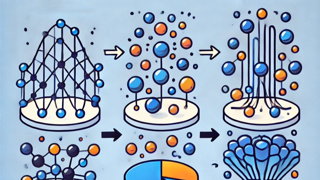
AdaBoost (Adaptive Boosting) is one of the most popular ensemble learning algorithms. It was introduced by Yoav Freund and Robert Schapire in 1996 as a method to combine multiple weak classifiers into a single strong classifier. Unlike bagging, which trains multiple classifiers independently, boosting focuses on sequentially improving weak classifiers by adjusting their weights.

Key Applications of AdaBoost

• Face Recognition (e.g., Viola-Jones algorithm)
• Text Classification (e.g., spam filtering)
• Anomaly Detection
• Medical Diagnosis and Disease Prediction

The Mathematics Behind AdaBoost

1. Assigning Initial Weights

Each training sample (x , y) is initially given an equal weight:

where is the total number of samples.

2. Training Weak Learners

A weak learner (often a decision stump) is trained on the weighted dataset. The weighted error of the weak learner is computed as:

where:

3. Determining Weak Learner’s Strength

he weak learner’s weight (alpha) is computed as:

4. Updating Sample Weights

Misclassified samples receive higher weights for the next iteration:

5. Constructing the Final Classifier

Step-by-Step Code Breakdown

1. Generating a Two-Circle Dataset

def generate_circles(n_samples=200, noise=0.15, factor=0.5, random_state=None):

This function generates a non-linearly separable dataset with two concentric circles:

• Outer Circle: Class +1
• Inner Circle: Class -1

 n_samples_out = n_samples // 2
  n_samples_in = n_samples - n_samples_out

Samples are split evenly between the two classes.

 theta_out = 2 * np.pi * np.random.rand(n_samples_out)
    r_out = 1.0 + noise * np.random.randn(n_samples_out)
    outer_x = r_out * np.cos(theta_out)
    outer_y = r_out * np.sin(theta_out)

Outer circle points are generated with radius ~1 and Gaussian noise.

 theta_in = 2 * np.pi * np.random.rand(n_samples_in)
    r_in = factor + noise * np.random.randn(n_samples_in)
    inner_x = r_in * np.cos(theta_in)
    inner_y = r_in * np.sin(theta_in)

 theta_in = 2 * np.pi * np.random.rand(n_samples_in)
    r_in = factor + noise * np.random.randn(n_samples_in)
    inner_x = r_in * np.cos(theta_in)
    inner_y = r_in * np.sin(theta_in)

Inner circle points are generated with a smaller radius, determined by factor.

 y = np.hstack([np.ones(n_samples_out), -np.ones(n_samples_in)])

Class labels are assigned: +1 for the outer circle, -1 for the inner circle.

2. Defining a Simple Decision Stump

class DecisionStump:
    def __init__(self):
        self.feature_index = None
        self.threshold = None
        self.polarity = 1

This class implements a basic one-level decision tree (stump).

def predict(self, X):
        predictions = np.ones(X.shape[0])
        if self.polarity == 1:
            predictions[X[:, self.feature_index] < self.threshold] = -1

Samples below the threshold are assigned class -1, based on polarity.

3. Training a Weighted Decision Stump

def train_decision_stump(X, y, weights):

This function trains a decision stump using weighted data.

 for feature_i in range(n_features):
        feature_values = X[:, feature_i]
        unique_values = np.unique(feature_values)

Every feature and all unique values are considered as possible thresholds.

for threshold in unique_values:
        for polarity in [1, -1]:

Both positive and negative polarities are tested to minimize error.

4. Implementing AdaBoost

class AdaBoost:
    def __init__(self, n_clf=10):

This class implements the AdaBoost classifier.

def fit(self, X, y, plot_progress=False):

This function:

1. Initializes sample weights.
2. Trains n_clf weak classifiers.
3. Updates sample weights.

 def predict(self, X):

The predict function aggregates all weak classifiers’ predictions.

5. Testing AdaBoost on a Complex Dataset

This section:

1. Generates a non-linearly separable dataset.
2. Trains AdaBoost with 20 weak classifiers.
3. Calculates model accuracy.

accuracy = np.sum(predictions == y) / len(y)
    print("Model accuracy on complex dataset: {:.2f}%".format(accuracy * 100))

The accuracy of the model is calculated and displayed.

Conclusion

• AdaBoost is a powerful ensemble method that converts weak learners into a strong classifier.
• It adjusts sample weights dynamically, focusing on harder-to-classify samples.
• This implementation demonstrates how AdaBoost handles complex, non-linearly separable data.

With this understanding, you can apply AdaBoost to real-world datasets and improve classification performance significantly! 🚀

For the complete code, visit my GitHub