ANOVA, Geometrically · Part 1 Why Your Data Is a Vector

Escaping the jungle of Σ symbols — one arrow at a time.

You already speak the language of statistics: means, variances, sums of squares, degrees of freedom. Each concept has its own formula and its own rules, and they seem to coexist as isolated, independent ideas. But the moment you try to derive anything in analysis of variance from first principles, you find yourself swallowed whole by a jungle of symbols — summations nested inside summations, subscripts multiplying out of control, two pages of algebra and still no end in sight.

This is not your fault. It’s the language’s fault.

The notation of statistics is an element-by-element language. Linear algebra offers a completely different one. Instead of processing elements one at a time, it treats an entire dataset as a single object — a vector — and operates on it as a whole. The theoretical foundations are complete and elegant. Translating a statistics problem into a linear algebra problem doesn’t just compress the notation; more importantly, it unlocks geometric intuition. In vector space, the statistical notions of “summation,” “mean,” and “variance” map perfectly onto the linear-algebraic notions of “inner product,” “projection,” and “magnitude (norm).”

We will stop thinking of data as “a collection of isolated numbers,” and start seeing them as a single vector living in high-dimensional space. This is a shift in perspective.

Data as Vectors

Column vectors: stand your data upright

Suppose you have exam scores for three students:

In the language of statistics, this is “a sample,” written .

In the language of linear algebra, this is a single vector:

This vector lives in — three-dimensional space. It is simultaneously a point and an arrow shooting out from the origin. Each student occupies one dimension. Three students, three dimensions. Not three dots scattered along a number line — rather, one point placed in 3D space.

The statistical view has a fatal scaling problem. Plotting points on a number line grows messier in direct proportion to . At it’s still readable. At points start to overlap. At the number line becomes a smear of color and individual information is almost entirely lost. And even when you can see every point clearly, you only learn “where things cluster, where they spread out.” Points have positional relationships only, no directional ones. The expressive ceiling is low.

The linear algebra view is the opposite. As grows, the vector gains dimensions — but on your diagram there is always one arrow. Complexity is absorbed into the dimensionality rather than splattered across the canvas.

Here is the key insight: any two vectors, regardless of how many dimensions each inhabits, together span a subspace of at most 2 dimensions (unless they are collinear, in which case it degenerates to 1 dimension). This means:

No matter whether is 12 or 1,200, whenever you want to discuss the relationship between and — their angle, their projection, their distance — you can always “flatten” both vectors onto a single 2D plane, draw the picture in full, and lose not a single detail.

This is precisely the power of linear algebra’s geometric language. It isn’t approximating high dimensions — by choosing the right plane, it brings a high-dimensional problem exactly down to two dimensions for discussion. Spoiler: the essence of analysis of variance is a right triangle living inside that 2D plane.

In summary, the shift in mathematical perspective is everything:

Statistical View Vector View data points scattered on a number line vector in Each data value is an independent number Each data value is one coordinate of the vector Relationships between data are described by formulas Relationships between vectors are described by geometry

Row Vectors and the Data Matrix

When we have multiple groups of data, matrices enter the picture.

Suppose you are running an ANOVA experiment with 3 groups, each containing 4 observations:

Group 1 Group 2 Group 3 Group 4 5 7 6 8 9 11 10 12 3 5 4 6

In statistical language, this is “three samples, four observations each.”

In linear algebra, this table can be read in two ways:

Read by rows — each row is the data vector for one group:

Read by columns — stack all observations into one long vector:

In ANOVA, we almost always use the second reading — stack all observations into a single long column vector .

Why? Because what ANOVA does is: decompose this long vector into several mutually perpendicular pieces. The object being decomposed must be a vector. You cannot orthogonally decompose a table.

This is the first step of vectorization: to give geometric tools like “projection,” “orthogonal decomposition,” and “subspace” a proper stage to perform on. Without a unified , the entire geometric framework has nothing to stand on.

All observations from one experiment → a single vector

The Core Argument

The central logic of this piece is to push for a shift in thinking — from “algebraic summation” to “geometric space.” This change of perspective does more than compress notation; it reveals the geometric soul of statistical relationships.

No matter how large the sample size, the connection between data and model can always be exactly projected onto a two-dimensional plane. And to make that geometric analysis possible, ANOVA must first “stack” all observations into a single unified high-dimensional sample space.

This is the foundation for everything that follows — a right triangle, drawn once, that makes the whole theory click.

You already speak the language of statistics: means, variances, sums of squares, degrees of freedom. Each concept has its own formula and its own rules, and they seem to coexist as isolated, independent ideas. But the moment you try to derive anything in analysis of variance from first principles, you find yourself swallowed whole by a jungle of symbols — summations nested inside summations, subscripts multiplying out of control, two pages of algebra and still no end in sight.

This is not your fault. It’s the language’s fault.

The notation of statistics is an element-by-element language. Linear algebra offers a completely different one. Instead of processing elements one at a time, it treats an entire dataset as a single object — a vector — and operates on it as a whole. The theoretical foundations are complete and elegant. Translating a statistics problem into a linear algebra problem doesn’t just compress the notation; more importantly, it unlocks geometric intuition. In vector space, the statistical notions of “summation,” “mean,” and “variance” map perfectly onto the linear-algebraic notions of “inner product,” “projection,” and “magnitude (norm).”

We will stop thinking of data as “a collection of isolated numbers,” and start seeing them as a single vector living in high-dimensional space. This is a shift in perspective.

Data as Vectors

Column vectors: stand your data upright

Suppose you have exam scores for three students:

In the language of statistics, this is “a sample,” written .

In the language of linear algebra, this is a single vector:

This vector lives in — three-dimensional space. It is simultaneously a point and an arrow shooting out from the origin. Each student occupies one dimension. Three students, three dimensions. Not three dots scattered along a number line — rather, one point placed in 3D space.

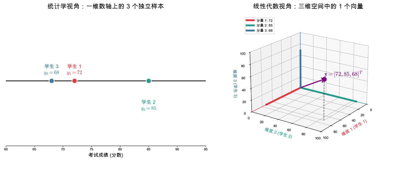
The statistical view has a fatal scaling problem. Plotting points on a number line grows messier in direct proportion to . At it’s still readable. At points start to overlap. At the number line becomes a smear of color and individual information is almost entirely lost. And even when you can see every point clearly, you only learn “where things cluster, where they spread out.” Points have positional relationships only, no directional ones. The expressive ceiling is low.

The linear algebra view is the opposite. As grows, the vector gains dimensions — but on your diagram there is always one arrow. Complexity is absorbed into the dimensionality rather than splattered across the canvas.

Here is the key insight: any two vectors, regardless of how many dimensions each inhabits, together span a subspace of at most 2 dimensions (unless they are collinear, in which case it degenerates to 1 dimension). This means:

No matter whether is 12 or 1,200, whenever you want to discuss the relationship between and — their angle, their projection, their distance — you can always “flatten” both vectors onto a single 2D plane, draw the picture in full, and lose not a single detail.

This is precisely the power of linear algebra’s geometric language. It isn’t approximating high dimensions — by choosing the right plane, it brings a high-dimensional problem exactly down to two dimensions for discussion. Spoiler: the essence of analysis of variance is a right triangle living inside that 2D plane.

In summary, the shift in mathematical perspective is everything:

Statistical View Vector View data points scattered on a number line vector in Each data value is an independent number Each data value is one coordinate of the vector Relationships between data are described by formulas Relationships between vectors are described by geometry

Row Vectors and the Data Matrix

When we have multiple groups of data, matrices enter the picture.

Suppose you are running an ANOVA experiment with 3 groups, each containing 4 observations:

Group 1 Group 2 Group 3 Group 4 5 7 6 8 9 11 10 12 3 5 4 6

In statistical language, this is “three samples, four observations each.”

In linear algebra, this table can be read in two ways:

Read by rows — each row is the data vector for one group:

Read by columns — stack all observations into one long vector:

In ANOVA, we almost always use the second reading — stack all observations into a single long column vector .

Why? Because what ANOVA does is: decompose this long vector into several mutually perpendicular pieces. The object being decomposed must be a vector. You cannot orthogonally decompose a table.

This is the first step of vectorization: to give geometric tools like “projection,” “orthogonal decomposition,” and “subspace” a proper stage to perform on. Without a unified , the entire geometric framework has nothing to stand on.

All observations from one experiment → a single vector

The Core Argument

The central logic of this piece is to push for a shift in thinking — from “algebraic summation” to “geometric space.” This change of perspective does more than compress notation; it reveals the geometric soul of statistical relationships.

No matter how large the sample size, the connection between data and model can always be exactly projected onto a two-dimensional plane. And to make that geometric analysis possible, ANOVA must first “stack” all observations into a single unified high-dimensional sample space.

This is the foundation for everything that follows — a right triangle, drawn once, that makes the whole theory click.