Building Regression Models in R using Support Vector Regression (SVR) — 2025 Update

Support Vector Regression (SVR) is a powerful machine learning technique for predicting continuous values, derived from the same principles that drive Support Vector Machines (SVM) in classification tasks.

In this article, we compare Simple Linear Regression (SLR) and SVR using the same dataset to illustrate how SVR can better handle non-linear relationships. We also walk through model tuning to improve predictive performance.

1. Quick Review: Simple Linear Regression (SLR)

SLR estimates the relationship between a dependent variable YYY and an independent variable XXX by fitting a straight line:

Y=α+βX+ϵY = \alpha + \beta X + \epsilonY=α+βX+ϵ

The parameters α\alphaα (intercept) and β\betaβ (slope) are estimated using the Ordinary Least Squares (OLS) method, which minimizes the sum of squared residuals.

Example in R

# Load tidyverse for modern data handling
library(tidyverse)

# Read CSV (ensure the file is in your working directory)
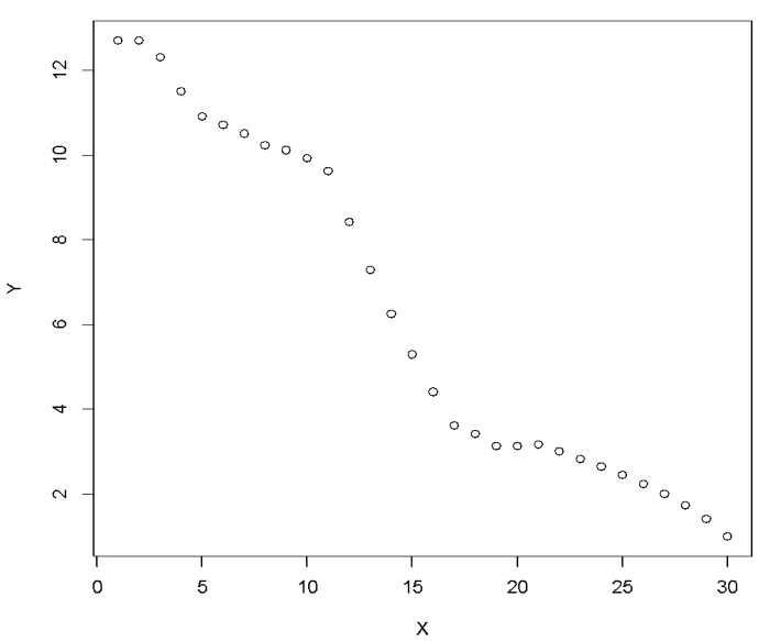
data <- read_csv("SVM.csv")

# Scatter plot
ggplot(data, aes(x = X, y = Y)) +
  geom_point(color = "black") +
  labs(title = "Scatter Plot of X vs Y") +
  theme_minimal()

# Fit SLR model
slr_model <- lm(Y ~ X, data = data)

# Add regression line
ggplot(data, aes(x = X, y = Y)) +
  geom_point() +
  geom_smooth(method = "lm", se = FALSE, color = "blue") +
  theme_minimal()

RMSE Calculation

In 2025, instead of hydroGOF, the yardstick package from the tidymodels ecosystem is preferred for model evaluation.

library(yardstick)

# Predictions
data <- data %>% mutate(pred_slr = predict(slr_model, .))

# RMSE
rmse(data, truth = Y, estimate = pred_slr)

2. Support Vector Regression (SVR)

SVR adapts the principles of SVM to regression problems. Key features:

• Kernel functions (Linear, Polynomial, Sigmoid, Radial Basis Function) allow modeling complex, non-linear relationships.
• Epsilon margin defines a tolerance zone where errors are ignored.
• Cost parameter © controls the penalty for predictions outside the epsilon margin.
• Less sensitive to the distributional assumptions required by linear regression.

Implementing SVR in R

For 2025, the e1071 package is still widely used, but many workflows now leverage the kernlab package for more advanced kernel methods and tidymodels for consistent syntax.

Using e1071 (classic approach)

library(e1071)

# Fit SVR with default RBF kernel
svr_model <- svm(Y ~ X, data = data, type = "eps-regression")

# Predictions
data <- data %>% mutate(pred_svr = predict(svr_model, .))

# RMSE
rmse(data, truth = Y, estimate = pred_svr)

3. Tuning the SVR Model

In 2025, hyperparameter tuning is most commonly done via tidymodels’ tune framework, but you can still use tune() from e1071.

Modern Tidymodels Example

library(tidymodels)

# SVR model specification
svr_spec <- svm_rbf(mode = "regression") %>%
  set_engine("kernlab")

# Cross-validation folds
set.seed(123)
folds <- vfold_cv(data, v = 5)

# Tuning grid
svr_grid <- grid_regular(cost(), rbf_sigma(), levels = 5)

# Workflow
svr_wf <- workflow() %>%
  add_model(svr_spec) %>%
  add_formula(Y ~ X)

# Tune
svr_tuned <- tune_grid(
  svr_wf,
  resamples = folds,
  grid = svr_grid,
  metrics = metric_set(rmse)
)

# Best parameters
best_params <- select_best(svr_tuned, "rmse")

# Final model
final_svr <- finalize_workflow(svr_wf, best_params) %>%
  fit(data)

4. Results Comparison

ModelRMSESLR0.94SVR (default)0.43Tuned SVR0.27

The tuned SVR model clearly outperforms both the SLR and untuned SVR models, especially on non-linear data.

5. Visualization of Model Fits

ggplot(data, aes(x = X)) +
  geom_point(aes(y = Y), color = "black") +
  geom_line(aes(y = pred_svr), color = "blue", size = 1) +
  geom_line(aes(y = predict(final_svr, new_data = data)$.pred),
            color = "red", linetype = "dashed", size = 1) +
  labs(title = "SLR vs SVR vs Tuned SVR",
       y = "Predicted Values") +
  theme_minimal()

6. Conclusion

• SLR is easy to implement but struggles with non-linear data.
• SVR handles non-linear relationships well via kernel tricks.
• Tuning SVR hyperparameters (cost, epsilon, sigma for RBF kernels) is crucial for best performance.
• In modern R workflows (2025), tidymodels provides a unified, consistent framework for modeling, tuning, and evaluation.

Recommendation:

• Use SLR for quick, interpretable models when relationships are mostly linear.
• Use SVR for complex, non-linear patterns—especially when predictive accuracy is the priority.

At Perceptive Analytics, we help organizations transform data into strategy through expert **tableau development services, dedicated guidance from an experienced [Power BI consultant](https://www.perceptive-analytics.com/microsoft-power-bi-developer-consultant/), and innovative [AI Consulting](https://www.perceptive-analytics.com/ai-consulting/)** for next-generation analytics solutions. With over two decades of experience, we empower businesses to make faster, smarter decisions.