Machine Learning : A Student Perspective

By Pratyush Jajodia

The Intuition: Why This Equation Matters

At its heart, y= mx+ b lays the foundation for the complex mathematics surrounding Machine Learning and its subset, Deep Learning.

The Equation of a Line

THE EQUATION OF A LINE (HIGH SCHOOL NOTATION)

• y: The output value.
• x: The input value.
• m: The slope (how steep the line is).
• b: The y-intercept (where the line crosses the vertical axis).

The Transition to Machine Learning Notation

Prediction with One Feature

This is just the fancy ML version of the high school line equation I talked about earlier.

• The Prediction (Hypothesis) H₀(x) : This is equivalent to the output (y). The goal of machine learning is to adjust weight and bias such that the prediction is close to the actual value
• The Bias (θ₀) : This is equivalent to intercept (b). The bias represents the model’s “starting point.” The value of y when x = 0 i.e. it represents what the prediction would be if all your input features were zero.
• The Weight (θ₁) : This is equivalent to Slope (m). The weight tells the model how much importance to give a specific feature. High Weight: A small change in the feature/ input (x) causes a massive change in the prediction (y). Zero Weight: The feature has no impact on the outcome. It’s effectively ignored. Negative Weight: As the feature increases, the prediction decreases (an inverse relationship).
• The Input (x₁) : This is equivalent to x (feature)

When you move from one feature to dozens, writing θ₀ + θ₁x₁ + θ₂x₂ + θ₃x₃ +… θₙxₙ becomes messy. This is why we use the vectorized form:

THE MATRIX NOTATION

Vectorized Form

In this version:

• x is a vector containing all input features (often with an extra “1” added to handle the intercept) representing all your data points.
• wᵀ is a vector containing all your weights for the features (θ₁ + θ₂+ ..θₙ)

The computer can calculate thousands of predictions simultaneously using linear algebra, which is much faster than calculating them one by one.

A example of different types of Lines :

1. The value of y when x = 0 i.e. it represents what the prediction would be if all your input features were zero.

The Bias Line

2. For the weights of features with non-zero values this is what the best fit line would look like —

Line of Best Fit

The Difference Between One Sample and the Whole Dataset

1. Entire Dataset

Y=Xw+b is sometimes confused with Y = wX + b but they are not the same. We know that matrix multiplication is not commutative in general: for matrices usually AB≠BA.

Let us consider a scenario of predicting height of M people using N features

• X = Feature matrix Shape (M X N)

m = number of examples (rows)
n = number of features (columns)

• w = Weight vector :(N ×1)
• b = Bias (Broadcasted to M ×1)
• Y = All predictions (M × 1)

MATRIX NOTATION

Understanding Weights (Size = Number of Features):

We know that each feature needs exactly one weight. Consider predicting height from age, weight, and income (3 features):

Total weights needed: 3 (one per feature). The weight dimensions are independent of the number of samples and only depend on the number of features.

Understanding Bias (Size = Broadcasted to Number of Samples):

While there is only one bias parameter learned for the layer, each prediction needs its own output. Therefore, that single bias term is “broadcasted” (copied) to be added to every single sample row.

2. One Sample Data

Dataset / matrix view:

In ML, usually we store the features as 1 X N (row vector)

Single sample: X∈R¹ˣᴺ (one row, N features)
Weights: w∈Rᴺˣ¹ (column vector).
Product: Xw ∈ (1×N)(N×1)=1×1

As a result we get a scalar prediction y. 

Algebra View:

We often treat vectors as column vectors by convention( ℝⁿ is treated as N X 1 ). This is why you sometimes see the notation y = wᵀx + b.

• w and x are column vectors
• wᵀ is a row vector.​

The Two Notations

The Moral Takeaway

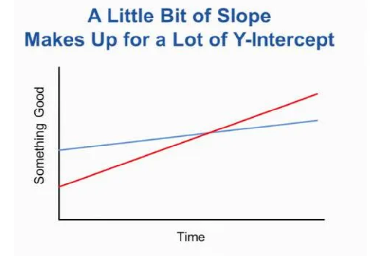
Learnings From the Equation

The slope is more important than the y-intercept. Regardless of your starting point (y-intercept), you will outperform everyone if you have the highest growth rate i.e., the slope. (Assuming it is not a negative slope, lol).

The Conclusion

I know one might wonder why I am obsessed with a simple equation; it ain’t that deep. But not just this, all the math concepts from linear algebra, calculus, and probability finally make sense as they come together in Machine Learning. Most importantly, its use case finally makes sense.