Want to know the adjacent points on road network and measure spacing? Try AdjFind

Consider a point dataset that can be mapped in the geographic space. For each point, we may want to know its neighboring points. The classic technique will be k-nearest neighbor query where k is a positive integer number such as 1, 2, or more; the query returns up to the user-defined amount of points that have the smallest Euclidean (straight-line) distances to the given point. Such a technique does not take road network into account, but in the real world travel happens along the road network; points that are deemed as nearest in Euclidean distance often are not true nearest in network distance. To get the k-nearest points in the network distance, one possibility will be computing the distance matrix using the point dataset and the road network, and extract the k+1 columns (one extra column that has the same point as origin and destination) with the smallest distance values for each row.

However, the neighboring points identified by k-nearest neighbor query or distance matrix really are proximity-based rather than adjacency-based. The figure below illustrates the difference: the black outline depicts land parcel boundaries, and blue polygons are single-family housing. For building 3, building 2 is to its left, and building 4 is to its right; buildings 2 and 4 are adjacent to building 3. However, building 1 is closer (or have same distance) to building 3 compared with building 4; 2-nearest neighbor query likely will return polygon 1 and 2. Therefore, there is a subtle difference between the results of proximity-based techniques and the expectations of a true adjacency-based technique.

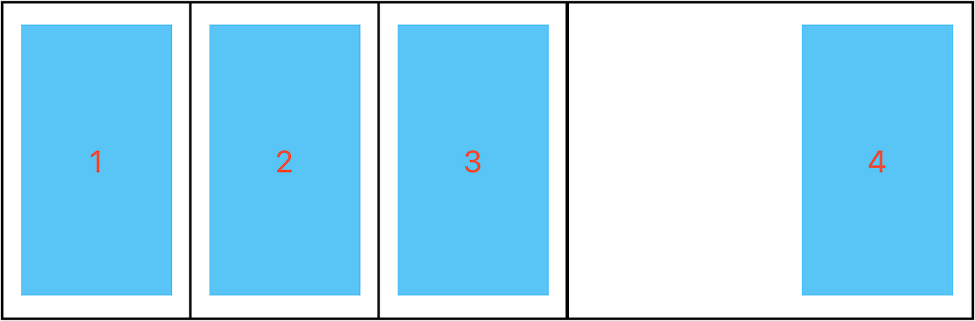
Figure 1

While proximity-based techniques are suitable for neighbor-identifications in most applications, adjacency-based techniques are still needed in certain applications. Spatial predicates such as touches or intersects can be used to determine adjacency relationship among polygons. In the figure above, the parcel where building 3 is located touches the parcels corresponding to building 2 and 4. However, for a dataset with non-duplicate points, directly applying spatial predicates will not work because there is always a positive amount of distance between any pair of points. Some GIS analysts might use buffer operation to convert points to polygons and then apply spatial predicates. There are three limitations of buffering the points: (i) it is often challenging to tell the appropriate buffer distance to set for the buffer operation; (ii) the neighboring points identified by buffer becomes coverage-based rather than adjacency-based (i.e., all the points within a distance threshold value will be considered as neighbors); (iii) buffering is an Euclidean-distance based operation that does not consider road network.

So far, I mention 3 similar and often interchangeable words: proximity, coverage, and adjacency. They can all be used to answer one question: what are the neighboring points of a given point? Those 3 words can be differentiated by how the concept of “neighbor” is defined.

1. A point is the neighbor of another point if it is the closest one or few points. I tend to use proximity (think about k-nearest neighbor query) to reference such applications.
2. A point is the neighbor of another point if it is within a distance threshold from the other point. I tend to use coverage (think about buffer + intersects) to reference such applications.
3. A point is the neighbor of another point if the shortest path between them is no longer than the shortest path to any other point in that travel direction. I tend to use adjacency to reference such applications. This concept is closely related to spacing (example will be hydrant spacing regulations), and it is not well-studied until recently by Figueroa et al. (2024).

In this article, I will take a deep dive into the third application category. While the focus will be point dataset rather than polygon dataset, I want to start with the Figure 1 that I discuss earlier. Assuming building 3 is the source, and we try to find its adjacent neighbors. If going straight to the left, we reach building 2. If continue going left, we can reach building 1 but the shortest path to building 1 is longer than the shortest path to building 2. Therefore, for this particular direction, building 2 is the adjacent neighbor while building 1 is not. There is another direction in which we can explore, which is to the right, and we can reach building 4, an adjacent neighbor in right-ward direction.

Figueroa et al. (2024) states the same approach in a more technical way. Imagine that we have computed the shortest paths from a source hydrant point to all other hydrant points in the dataset, “if an edge on a path from hydrant i to hydrant l is closer to a hydrant other than i, the path is discarded, and the candidate neighbor is excluded.” In fact, this article as well as the AdjFind neighboring-points mode are stemmed from Figueroa et al. (2024); for any future academic literature that plan to cite the related works, please cite Figueroa et al. (2024) accordingly.

The following figures should illustrate the concept more clearly. Imagine a point that is snapped to the middle of a west-east-oriented road line-string. There are two possible directions of travel along the road line-string: going left or going right. If going left, as soon as the shortest path to another point is found, the search in the left direction can terminate. Basically, rather than calculating the paths to all other points and discarding paths to non-adjacent points, revising the path algorithm itself will be an more efficient approach. Similarly, another run of the specialized path algorithm going right will give us the second adjacent neighbor.

Figure 2

Figure 3

If the point is located very close to the road intersection, its possible travel directions may not be limited to just two since it effectively can be treated as at the intersection (Figueroa et al. (2024)). The following figures illustrate that left-direction can be further split to left-left, left-up, and left-down directions.

Figure 4

Figure 5

AdjFind is a C++ command line application that is capable to identify adjacent point neighbors and the corresponding spacing distances. If the application problem that you try to solve defines the concept of neighbor in the same way as AdjFind, you got a readily available tool to use now! If you like this work, please star or fork the GitHub repository.

If you are interested in knowing more about the capability of AdjFind, feel free to read my previous article.

If you want to learn the path algorithm used in the neighboring-points mode of AdjFind, please read the following section.

The path algorithm assumes a weighted graph constructed in the same manner as the Constructing graph with points snapped section of my previous article. It is a variant of Dijkstra algorithm with following key differences:

1. The termination criteria is: the current vertex (the vertex that is just finalized or labeled) has a vertex type of point (the graph vertices created from input data’s road intersections will have type intersection, while graph vertices that correspond to the input point dataset will have type point) and is not the source vertex (source vertex will always have type point because the overall algorithm loops through each point sourced from the point dataset). This ensures that no further branching as soon as another point vertex is reached.
2. An extra vector edges_to_exclude is introduced. In the code block that iterates through each outgoing edges (or connected vertices) of the current vertex, if the outgoing edge is in the edges_to_exclude vector, it will continue to next iteration instead of adding the corresponding connected vertex to the priority queue. Visually, this parameter serves like the forbidden symbols in figure 2 and 4; for example, if I want to find the adjacent neighbor to the left, I will add the edge on the right to the edges_to_exclude vector, so that the path is restricted to go left. I call this strategy as restricted directional search.

For each point (e.g., hydrant) vertex in the graph, the general flow is like following (the function call refers to the path algorithm described above):

Figure 6

Note the third decision box (yellow box) addresses the following special situation that has more than one hydrant near the intersection:

Figure 7

Hydrant vertex 5 is very close to intersection vertex 4, should it make multiple path algorithm function calls to take upward direction into account? No, because intersection vertex 4 has two hydrant vertices nearby. A single function call that will return a path ended at vertex 6 will be sufficient for the upward direction.

That is it! Now you know the fundamentals of the algorithms underlying the AdjFind neighboring-points mode!