CNN Image Classification TensorFlow for 30 Musical Instruments

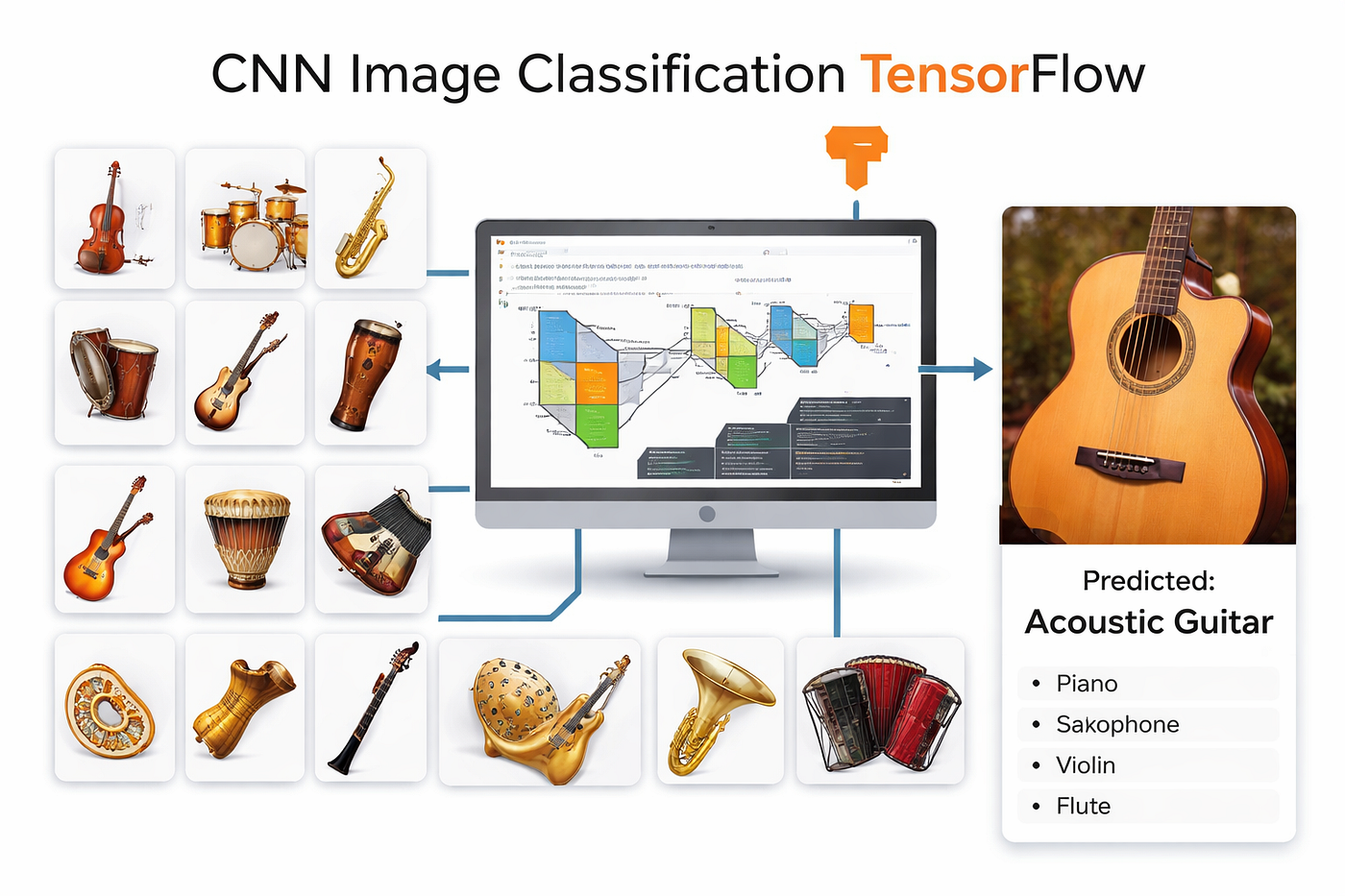
I wanted a model that can look at a single image and confidently say “accordion”, “violin”, or “saxophone” — not by guessing, but by learning real visual patterns. That’s exactly what this cnn image classification tensorflow tutorial builds: a complete workflow for training a custom CNN to recognize 30 musical instrument classes from images.

Instead of focusing only on layers, this walkthrough focuses on the whole pipeline that makes training feel reliable: loading data from a folder structure, feeding it efficiently into TensorFlow, saving the best model automatically, and then proving performance with a confusion matrix and a per-class classification report.

If you’ve trained a model before and felt unsure whether it’s truly learning (or just memorizing), this tutorial is designed to remove that uncertainty. You’ll see how to verify the dataset early, how to stabilize training, and how to evaluate results in a way that highlights exactly which instruments your CNN confuses.

If you want the dataset layout I used so you can reproduce the same experiment more easily, email me at feitgemel@gmail.com and include the subject: “30 Musical Instruments CNN dataset”.

What this CNN project will actually do

By the end, you’ll have a working cnn image classification tensorflow pipeline that:

• Loads images from train/, valid/, and test/ folders (30 subfolders = 30 classes).
• Trains a CNN with convolution + pooling + dense layers.
• Uses early stopping and model checkpoints to reduce overfitting.
• Predicts a random test image like a real user scenario.
• Evaluates every test image and visualizes a confusion matrix.
• Prints a classification report so you can see per-class precision/recall.

If you want the dataset layout I used so you can replicate the same setup, email me with the subject: “30 Musical Instruments CNN dataset”.

Building a CNN pipeline to recognize 30 musical instruments

This tutorial walks through a complete, code-first pipeline for training a Convolutional Neural Network (CNN) with TensorFlow to classify 30 musical instrument classes from images. The focus is not just on defining layers, but on creating a reliable workflow: loading a structured dataset, preprocessing images, training with safeguards against overfitting, and evaluating performance with meaningful metrics.

At its core, the code demonstrates how to transform raw image folders into a high-performance training pipeline using image_dataset_from_directory, normalization, caching, and prefetching. These steps ensure that the GPU or CPU stays fed with data efficiently, reducing bottlenecks and making training smoother. By structuring the dataset into train, validation, and test directories, the pipeline mirrors real-world machine learning workflows used in production.

The CNN architecture itself is designed to balance performance and generalization. Convolutional layers progressively extract visual features such as edges, shapes, and textures that distinguish instruments like guitars, violins, and saxophones. Pooling layers reduce spatial complexity, while dense layers interpret the extracted features to produce a final prediction across 30 classes. Dropout layers add regularization, helping the model avoid memorizing the training data.

Training is guided by practical safeguards that make the code suitable for real projects. Early stopping halts training when validation performance stops improving, preventing wasted computation and overfitting. Model checkpoints ensure that the best-performing version of the network is saved automatically. After training, the evaluation phase goes beyond accuracy by generating a confusion matrix and classification report, revealing which instruments are commonly misclassified and providing actionable insight for further improvements.

[embed]

Link to the video tutorial here

Download to the code for the tutorial here or here

My Blog

You can follow my blog **here **.

Link to the full post and code : https://eranfeit.net/cnn-image-classification-tensorflow-30-musical-instruments/

Want to get started with Computer Vision or take your skills to the next level ?

Great Interactive Course : “Deep Learning for Images with PyTorch” here

If you’re just beginning, I recommend this step-by-step course designed to introduce you to the foundations of Computer Vision — Complete Computer Vision Bootcamp With PyTorch & TensorFlow

If you’re already experienced and looking for more advanced techniques, check out this deep-dive course — Modern Computer Vision GPT, PyTorch, Keras, OpenCV4

Best AI Photo Tools (Backgrounds, Objects, Headshots)

✅ Phot-AI packs more than 30 AI‑powered tools into one place — covering background and object removal/replacement, image extension and a suite of creative generators for art, icons and logos.

follow the link and start creating : https://phot.ai?ref=eran33

✅ Pixelcut uses AI to help you create professional photos and videos. You can instantly remove backgrounds, retouch, expand and upscale images, or generate new images and even videos from a simple text prompt or reference picture. tap the link and start creating today! : https://pixelcut.ai/?via=eran

✅ PhotoGPT AI acts as your personal photographer — just describe what you need and the platform generates high‑quality headshots or casual images within minutes.

Its built‑in photo editor lets you remove objects, replace backgrounds and make studio‑quality corrections with a single click.

You can even train your own AI model using a few selfies, receive context‑aware prompt suggestions and upscale images for print‑ready results.

Dive into this all‑in‑one AI photo studio : https://www.photogptai.com/?ref=eran

Part A: Environment setup that prevents “random” TensorFlow issues

Before any modeling, it’s worth locking your environment down. Small version mismatches can cause GPU detection problems, slow training, or confusing runtime errors. Creating a dedicated environment makes the tutorial repeatable.

The installs below are intentionally specific. When you train and evaluate, you want consistent behavior across sessions — especially when you later compare results after changing model structure or training parameters.

If you’re on GPU, make sure your TensorFlow build matches your CUDA setup. If you’re on CPU, keep it simple and focus on correctness first.

conda create -n TASM python=3.11 
conda activate TASM 

nvcc --version

# For GPU users for Cuda 12.3 
pip install tensorflow[and-cuda]==2.17.1

# For CPU users
pip install tensorflow==2.17.1

pip install numpy==1.26.4
pip install matplotlib==3.10.0
pip install pandas==2.2.3
pip install scikit-learn==1.6.0
pip install seaborn==0.13.2
pip install opencv-python==4.10.0.84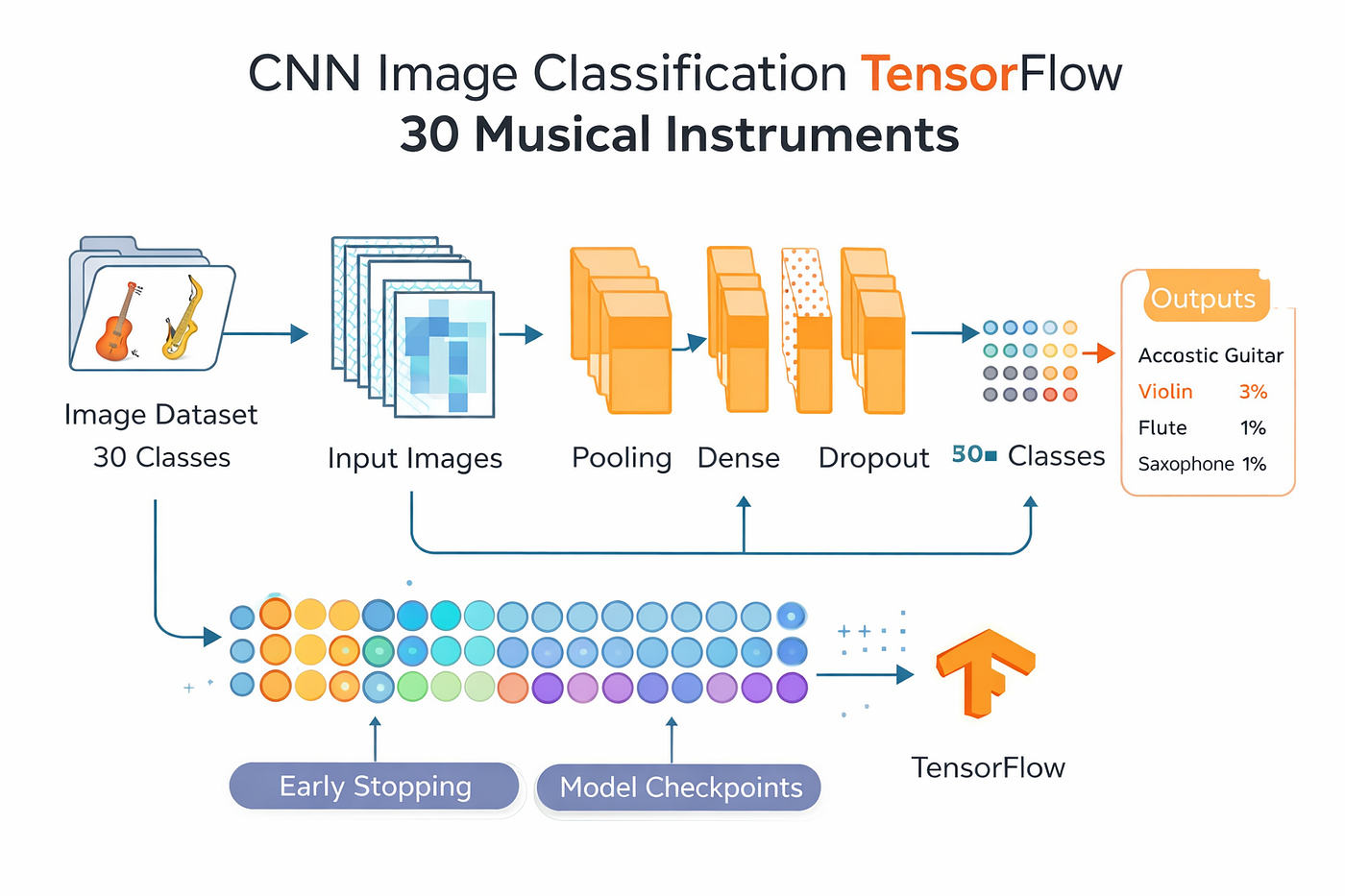

Part B: Sanity-check the dataset and define your training settings

A reliable pipeline starts with verifying the basics: paths, image size, and whether a real image loads correctly. This tiny step saves you from training for an hour only to discover a path typo or a shape mismatch.

The image size here is set to 128×128 to keep training lightweight and fast. It’s a great choice for learning and iteration. If you later want more detail (and you have enough data), you can increase it.

This also sets up the main training parameters — batch size and epochs — so the entire run is easy to control and reproduce.

import numpy as np
import pandas as pd
import matplotlib.pyplot as plt

from keras.utils import img_to_array, load_img
from keras.callbacks import EarlyStopping, ModelCheckpoint
from tensorflow.keras.optimizers import Adam

import tensorflow as tf
from tensorflow.keras.models import Sequential
from tensorflow.keras.layers import Dense, Flatten, Conv2D, MaxPooling2D, Dropout

# Paths and parameters
train_path = '/mnt/d/Data-Sets-Image-Classification/30 Musical Instruments/train/'
valid_path = '/mnt/d/Data-Sets-Image-Classification/30 Musical Instruments/valid/'

BATCH_SIZE = 8
IMG_SIZE = (128,128)
IMG_DIM = (128,128,3)
EPOCHS = 200 

# Display a sample image 
img = load_img(train_path + 'acordian/010.jpg') 
plt.imshow(img)
img = img_to_array(img)
print(img.shape)
plt.show()

Part C: Build a fast tf.data input pipeline from folder structure

This is where TensorFlow starts to feel like a real production workflow. image_dataset_from_directory builds a dataset directly from your folder structure, creates integer labels, resizes images, batches them, and shuffles them.

Then you normalize pixel values into [0,1]. This simple normalization step makes optimization far more stable and helps the model learn with fewer surprises.

Finally, caching and prefetching reduce bottlenecks. If your GPU is waiting for disk reads, training looks slow and “broken.” This keeps the pipeline flowing smoothly.

# Load the dataset :
train_dataset = tf.keras.utils.image_dataset_from_directory(
    train_path,
    image_size=IMG_SIZE,
    batch_size=BATCH_SIZE,
    shuffle=True,
    label_mode='int'
)

valid_dataset = tf.keras.utils.image_dataset_from_directory(
    valid_path,
    image_size=IMG_SIZE,
    batch_size=BATCH_SIZE,
    shuffle=True,
    label_mode='int'
)

# Normalize the pixel values to [0, 1]
def normalize(image, label):
    return tf.cast(image, tf.float32) / 255.0, label

train_dataset = train_dataset.map(normalize)
valid_dataset = valid_dataset.map(normalize)

# Cache and prefetch the datasets for performance
AUTOTUNE = tf.data.AUTOTUNE
train_dataset = train_dataset.cache().prefetch(buffer_size=AUTOTUNE)
valid_dataset = valid_dataset.cache().prefetch(buffer_size=AUTOTUNE)

Part D: The CNN architecture for 30 instrument classes

A good baseline CNN doesn’t need to be complicated. This model uses a classic pattern:

• Convolutions learn visual features (edges → textures → parts of instruments).
• Pooling compresses the representation and adds robustness.
• Dense layers combine features into a final decision.
• Dropout reduces overfitting risk.
• Softmax outputs probabilities across 30 classes.

This is a strong starting point for a cnn image classification tensorflow project. If you later want a major accuracy upgrade, transfer learning is the next step — but starting with a readable CNN teaches you what’s happening.

# Build the CNN model

def get_cnn_model():
    model = Sequential()

    model.add(Conv2D(32, kernel_size=3 , padding='same', activation='relu', input_shape=IMG_DIM)) 
    model.add(MaxPooling2D((3,3)))
    model.add(Conv2D(64, kernel_size=3 , padding='same', activation='relu'))
    model.add(MaxPooling2D((3,3)))
    model.add(Conv2D(128, kernel_size=3 , padding='same', activation='relu'))
    model.add(Flatten())
    model.add(Dense(256, activation='relu'))
    model.add(Dropout(0.5))
    model.add(Dense(128, activation='relu'))
    model.add(Dropout(0.5))
    model.add(Dense(30, activation='softmax'))
    model.compile(optimizer=Adam(learning_rate=0.001), loss='sparse_categorical_crossentropy', metrics=['accuracy'])
    return model

model = get_cnn_model()
print(model.summary())

Part E: Train with checkpoints + early stopping (save the best model)

This section is what separates casual training from a reliable workflow.

• ModelCheckpoint saves the best model automatically based on validation loss.
• EarlyStopping stops training when the model stops improving, reducing overfitting and saving time.

You also plot training curves at the end. These plots are extremely useful. If validation loss rises while training loss drops, you’re likely overfitting.

# Save the best model during training using ModelCheckpoint
check_point_path = "/mnt/d/models/Best-CNN-Model-30-Musical-Instruments.keras"
checkpoint_callback = ModelCheckpoint(
    filepath=check_point_path,
    monitor='val_loss',
    save_best_only=True,
    verbose=1
)

# Early stopping to prevent overfitting
erly_stopping_callback = EarlyStopping(monitor='val_loss', patience=40, verbose=1) 

# Train the model
history = model.fit(
    train_dataset,
    validation_data=valid_dataset,
    epochs=EPOCHS,
    callbacks=[checkpoint_callback, erly_stopping_callback]
)

# Save the final model
model.save('/mnt/d/models/Final-CNN-Model-30-Musical-Instruments.keras')

# Plot training & validation accuracy and loss values
acc = history.history['accuracy']
val_acc = history.history['val_accuracy']
loss = history.history['loss']
val_loss = history.history['val_loss']

epochs_range = range(len(acc))

plt.figure(figsize=(12, 6))
plt.subplot(1, 2, 1)
plt.plot(epochs_range, acc, label='Training Accuracy')
plt.plot(epochs_range, val_acc, label='Validation Accuracy')
plt.legend(loc='lower right')
plt.title('Training and Validation Accuracy')

plt.subplot(1, 2, 2)
plt.plot(epochs_range, loss, label='Training Loss')
plt.plot(epochs_range, val_loss, label='Validation Loss')
plt.legend(loc='upper right')
plt.title('Training and Validation Loss')

plt.show()

Part F: Predict a random test image + evaluate everything with a confusion matrix

This is where the tutorial becomes “real world.”

First, you load the saved best model and predict a random image from the test dataset. This quick test is a sanity check and a great way to spot obvious preprocessing mistakes.

Then you evaluate every test image and build a confusion matrix. With 30 classes, the confusion matrix is often more informative than accuracy. It shows exactly which instruments the CNN confuses.

Finally, the classification report prints precision, recall, and F1 per class, which is critical when some classes have fewer images or are visually similar.

import os 
import random
import numpy as np
import tensorflow as tf
import cv2 
import matplotlib.pyplot as plt
from sklearn.metrics import classification_report, confusion_matrix
import seaborn as sns

test_path = '/mnt/d/Data-Sets-Image-Classification/30 Musical Instruments/test/'
model_path = "/mnt/d/models/Best-CNN-Model-30-Musical-Instruments.keras"

IMG_SIZE = (128,128)
class_names = sorted(os.listdir(test_path))
print(class_names)

# Load the trained model
model = tf.keras.models.load_model(model_path)
print("Model loaded successfully.")

# Task 1 - Predict a random image from the test folder 

def predict_random_image():
    # Select a random class folder 
    random_class = random.choice(class_names)
    class_folder = os.path.join(test_path, random_class)

    # Select a random image from the class folder
    random_image = random.choice(os.listdir(class_folder))
    image_path = os.path.join(class_folder, random_image)

    # load the image using Opencv
    image = cv2.imread(image_path)
    image_rgb = cv2.cvtColor(image, cv2.COLOR_BGR2RGB)

    # Preprocess the image
    image_resized = cv2.resize(image_rgb, IMG_SIZE)
    input_array = np.expand_dims(image_resized / 255.0, axis=0)  # Normalize and add batch dimension

    # Prediction
    predictions = model.predict(input_array)
    predicted_class_index = np.argmax(predictions) 
    predicted_class = class_names[predicted_class_index]

    # Dsiplay the image with predicted label
    plt.figure(figsize=(6,6))
    plt.imshow(image_rgb)
    plt.title(f"Predicted: {predicted_class}\nTrue Class: {random_class}", fontsize=14)
    plt.axis('off')
    plt.show()

# Run the prediction function (random image)
predict_random_image()

# -----------------------------------------------------------------
# Task 2 : Predict all images in the test folder and display a confusion matrix

def evaluate_model():
    true_labels = []
    predicted_labels = []

    for class_index , class_name in enumerate(class_names):
        class_folder = os.path.join(test_path, class_name)
        for image_name in os.listdir(class_folder):
            image_path = os.path.join(class_folder, image_name)

            # Load and preprocess the image
            image = cv2.imread(image_path)
            image_rgb = cv2.cvtColor(image, cv2.COLOR_BGR2RGB)
            image_resized = cv2.resize(image_rgb, IMG_SIZE)
            input_array = np.expand_dims(image_resized / 255.0, axis=0)  # Normalize and add batch dimension

            # Prediction
            predictions = model.predict(input_array)
            predicted_class_index = np.argmax(predictions)

            # Append true and predicted labels
            true_labels.append(class_index)
            predicted_labels.append(predicted_class_index)

    # Generate confustion matrix
    cm = confusion_matrix(true_labels, predicted_labels)

    # Visualize the confusion matrix
    plt.figure(figsize=(12,8))
    sns.heatmap(cm, annot=True, fmt='d', xticklabels=class_names, yticklabels=class_names) 
    plt.xlabel('Predicted Label')
    plt.ylabel('True Label')
    plt.title('Confusion Matrix')
    plt.show()

    # Classification report
    report = classification_report(true_labels, predicted_labels, target_names=class_names)
    print("Classification Report:\n", report)
    print(f"Evaluated class: {class_name}")

# Run the evaluation function
evaluate_model()

Practical notes that help this model improve faster

If validation accuracy stalls early, the most common cause is not the architecture — it’s the dataset. Similar instruments, similar backgrounds, and inconsistent lighting can make classes hard to separate.

If you want a quick improvement path, focus on three things first:

1. more image variety per class,
2. consistent preprocessing,
3. adding augmentation (later) once the baseline pipeline is confirmed stable.

The confusion matrix is your compass. If two instruments are frequently confused, that tells you exactly which classes need more examples or more variety — not a random global change.

Wrap-up

This cnn image classification tensorflow pipeline gives you something you can reuse: folder-based datasets, efficient TensorFlow loading, a clean CNN baseline, controlled training with checkpoints, and evaluation that reveals what the model is really learning.

Once you’re comfortable with this structure, you can scale it in multiple ways: increase image resolution, try transfer learning, add augmentation, or deploy the trained model for faster inference. But the foundation stays the same — and that foundation is what makes your results dependable.

Connect :

☕ Buy me a coffee — https://ko-fi.com/eranfeit

🖥️ Email : feitgemel@gmail.com

🌐 https://eranfeit.net

🤝 Fiverr : https://www.fiverr.com/s/mB3Pbb

Enjoy,

Eran