Navigating Credit Risk: Measuring Potential Future Exposure for SOFR Swaps with the Hull-White Model in QuantLib Python

A practical guide to simulating interest rates, repricing swaps, and quantifying counterparty credit risk.

Introduction for Potential Future Exposure

Introduction

In the complex world of financial derivatives, managing counterparty credit risk is paramount. One crucial metric for this is Potential Future Exposure (PFE), which provides a forward-looking view of the maximum possible loss due to a counterparty’s default. This article will delve into PFE, its importance in credit risk management, and demonstrate how to calculate it for a SOFR swap using the Hull-White interest rate model within QuantLib Python. We will also touch upon additional real-world considerations when calculating PFE.

So, what is Potential Future Exposure (PFE)?

Potential Future Exposure (PFE) represents the maximum expected credit exposure to a counterparty at a given future date, within a specified confidence level. Unlike current exposure, which reflects the immediate mark-to-market value of a derivative portfolio, PFE is a probabilistic measure. It considers various market scenarios to project the potential positive value of a derivative contract (or portfolio) if interest rates, exchange rates, or other underlying assets move adversely.

In essence, if a counterparty defaults, and your derivative contract with them has a positive value (meaning they owe you money), then that positive value represents your exposure. PFE aims to quantify the “worst-case” scenario for this exposure at different points in the future.

How Do Market Participants Use PFE to Monitor Credit Risk?

Market participants, particularly banks and financial institutions, utilize PFE in several critical ways to monitor and manage credit risk:

• Setting Credit Limits: PFE is a key input for establishing bilateral credit limits with counterparties. By understanding the potential future exposure, institutions can set appropriate limits to ensure they are not overexposed to any single entity.
• Collateral Management: PFE helps in determining initial margin requirements for uncollateralized or partially collateralized trades. Higher PFE often necessitates higher collateral to mitigate potential losses.
• Capital Allocation: Regulatory frameworks (like Basel III) require financial institutions to hold capital against their credit exposures. PFE calculations feed into these capital adequacy requirements, ensuring sufficient capital reserves to absorb potential losses from counterparty defaults.
• Risk Reporting and Stress Testing: PFE figures are crucial for internal risk reporting and stress testing scenarios. By simulating extreme market movements, institutions can assess the resilience of their portfolios and identify potential vulnerabilities.
• Pricing Derivatives: While not directly used in the base pricing of a derivative, the cost of counterparty credit risk (often linked to PFE) can be incorporated into the overall pricing framework, especially for long-dated or complex trades.

Using the Hull-White Interest Rate Model to Simulate Interest Rates and Value PFE with QuantLib Python

To calculate PFE, we can simulate future interest rate paths and revalue our SOFR swap under each path. The Hull-White model is a popular choice for this as it’s an analytically tractable single-factor short-rate model that allows for calibration to the yield curve.

Let’s walk through a simplified example using QuantLib Python.

First, import library and setup reference valuation date.

import QuantLib as ql
from datetime import datetime
import pandas as pd
import numpy as np

# 1. Set up the evaluation date
today = ql.Date(15, 4, 2025)
ql.Settings.instance().evaluationDate = today

Define the market environment, load USD SOFR zero curve that has been created and initialize SOFR Index.

day_count = ql.Actual360()
calendar = ql.UnitedStates(ql.UnitedStates.GovernmentBond)

# ---simple function to help convert to QuantLib Date ---
def to_ql_date(date_str):
    date_obj = datetime.strptime(date_str, "%m/%d/%Y")
    return ql.Date(date_obj.day, date_obj.month, date_obj.year)

# load USDSOFR zero rate curve
df_usdsofr_curve = pd.read_csv('usd_sofr_curve.csv')
# Apply conversion
df_usdsofr_curve['QL_Date'] = df_usdsofr_curve['Date'].apply(to_ql_date)
curve_dates = df_usdsofr_curve['QL_Date'].tolist()
curve_zeros = [value/100 for value in df_usdsofr_curve['ZeroRate']]

usd_sofr_curve_data = ql.ZeroCurve(curve_dates, 
                          curve_zeros, 
                          ql.Actual365Fixed(), 
                          calendar)

pricing_curve_handle = ql.RelinkableYieldTermStructureHandle(usd_sofr_curve_data)

# Initialize SOFR index to the curve
sofr_index = ql.Sofr(pricing_curve_handle)

Create a 5-Year SOFR Swap trade with notional amount 10 million and swap rate 4%.

usd_notional = 10000000.0 # trade notional
fixed_rate = 0.04  # assume trade fixed rate 4.9%
swap_term = ql.Period('5Y') # trade term
start_date = ql.Date(17, 4, 2025) # trade effective date
maturity_date = start_date + swap_term # trade maturity date

# initialize SOFR 
sofr_index = ql.Sofr(pricing_curve_handle)

# fixed-leg schedule
fixed_schedule = ql.Schedule(
    start_date, maturity_date,
    ql.Period("1Y"), calendar,
    ql.ModifiedFollowing, ql.ModifiedFollowing,
    ql.DateGeneration.Forward, False
)
# sofr-leg schedule
float_schedule = ql.Schedule(
    start_date, maturity_date,
    ql.Period("1Y"), calendar,
    ql.ModifiedFollowing, ql.ModifiedFollowing,
    ql.DateGeneration.Forward, False
)
# define SOFR Swap trade
sofr_swap = ql.OvernightIndexedSwap(
    ql.Swap.Payer, # Swap.Payer means pay fixed coupon and receive floating coupon
    [usd_notional],
    fixed_schedule,
    fixed_rate,
    ql.Actual360(),
    [usd_notional],
    float_schedule,
    sofr_index,
    0.0,
    2) # Payment lag=2 for standard USD SOFR Swap trade.

Then we set the pricing engine to the Swap trade and get the NPV.

swap_engine = ql.DiscountingSwapEngine(pricing_curve_handle)
sofr_swap.setPricingEngine(swap_engine)
print(f"Swap NPV: {sofr_swap.NPV():.2f} USD")

Swap NPV: 1182.42 USD

Next, Let’s simulate interest rate paths for PFE Calculation.

# Define number of simulated paths
num_paths = 1000 
# Determine the total time span in years for the simulation
total_sim_time = 30
# Define time steps for simulation. It's often good to align with observation dates.
# Let's target quarterly steps for simulation, for finer granularity if needed.
num_steps = int(total_sim_time * 4) # E.g., 4 steps per year
times_grid = ql.TimeGrid(total_sim_time, num_steps) # Time grid for simulation

# For demonstration, we'll use assumed parameters.
# for how to calibrate 'a' and 'sigma' to market swaption volatilities could
# refer to preivous article.
a = 0.0324 # Mean reversion speed
sigma = 0.002335 # Volatility of the short rate

# Create a Hull-White process
hw_process = ql.HullWhiteProcess(pricing_curve_handle, a, sigma)

# Create a Gaussian path generator for the Hull-White proces
random_num_generator = ql.InvCumulativeMersenneTwisterGaussianRsg(
    ql.MersenneTwisterUniformRsg(num_steps, ql.MersenneTwisterUniformRng(42)))
seq_generator = ql.InvCumulativeMersenneTwisterPathGenerator(hw_process, times_grid, random_num_generator, False)

simulated_rates = np.zeros((num_paths, num_steps + 1))
for i in range(num_paths):
    path = seq_generator.next().value()
    for j in range(len(path)):
        simulated_rates[i, j] = path[j]

Convert time points to dates for observation_dates, ensuring they align with simulated path times. We need to map time_grid points to actual dates for evaluation.

observation_dates_ql = []
observation_times_ql = []
for t_idx, t_val in enumerate(times_grid):
    # Calculate the date corresponding to this time point
    # Add an epsilon to avoid floating point issues when comparing with actual dates
    obs_date_ql = today + ql.Period(int(t_val * 365.25), ql.Days)
    # Ensure obs_date_ql is not before today if t_val is 0.0
    if obs_date_ql < today:
        obs_date_ql = today

    # Store unique dates and their corresponding times in the original time grid
    # and ensure they are before maturity date
    # This avoids duplicates and ensures we only consider dates before maturity.
    if obs_date_ql not in observation_dates_ql and obs_date_ql < maturity_date:
        observation_dates_ql.append(obs_date_ql)
        observation_times_ql.append(t_val) # Store the actual time value from the grid

# Sort by date
sorted_indices = np.argsort([d.serialNumber() for d in observation_dates_ql])
observation_dates = [observation_dates_ql[i] for i in sorted_indices]
observation_times = [observation_times_ql[i] for i in sorted_indices]

Add current SOFR fixing rate and initialize another curve handler for Hull White process.

current_fixing_date = today
sofr_index.addFixing(current_fixing_date, 0.04) # Add fixing for the start date
sofr_curve_handle = ql.YieldTermStructureHandle(usd_sofr_curve_data)

Now, we start calculate PFE for the SOFR swap trade.

pfe_values = []
confidence_level = 0.95 # For 95% PFE (one-sided)

for obs_idx, obs_date in enumerate(observation_dates):
    # Set the evaluation date for the CURRENT ITERATION
    ql.Settings.instance().evaluationDate = obs_date
    swap_values_at_obs_date = []

    # add projected SOFR rates to historical fixings.
    while obs_date > current_fixing_date:
        next_fixing_date = sofr_index.fixingCalendar().advance(current_fixing_date, 1, ql.Days)
        fwd_sofr_rate = sofr_curve_handle.forwardRate(current_fixing_date, next_fixing_date, ql.Actual365Fixed(),ql.Compounded).rate()
        if not sofr_index.hasHistoricalFixing(current_fixing_date):
            sofr_index.addFixing(current_fixing_date, fwd_sofr_rate)
        current_fixing_date = next_fixing_date


    current_time_val = observation_times[obs_idx]
    sim_time_idx = np.where(np.isclose(times_grid, current_time_val, atol=1e-6))[0][0]

    for i in range(num_paths):
        simulated_short_rate_at_obs = simulated_rates[i, sim_time_idx]

        # --- Construct the simulated discount curve consistent with Hull-White ---
        sim_curve_dates = [obs_date]
        if obs_date < maturity_date:
            # Add dates up to or slightly beyond swap maturity
            # roughly quarterly steps
            for k in range(0, (maturity_date - obs_date) + 30, 90): 
                future_date = obs_date + ql.Period(k, ql.Days)
                if future_date > maturity_date:
                    future_date = maturity_date # Cap at maturity
                sim_curve_dates.append(future_date)
        # Remove duplicates and sort
        sim_curve_dates = sorted(list(set(sim_curve_dates)))
        # Ensure maturity date is included 
        sim_curve_dates.append(maturity_date+ql.Period(90, ql.Days)) 

        sim_discounts = []
        for d in sim_curve_dates:
            discount_factor = ql.HullWhite(sofr_curve_handle, a, sigma).discountBond(
                ql.Actual365Fixed().yearFraction(today, obs_date),  # Time from initial today to obs_date
                ql.Actual365Fixed().yearFraction(today, d),         # Time from initial today to target date d
                simulated_short_rate_at_obs # The short rate at obs_date
            )
            sim_discounts.append(discount_factor)

        # Create a discount curve from the simulated dates and discounts
        sim_discount_curve = ql.DiscountCurve(sim_curve_dates, sim_discounts, ql.Actual365Fixed())

        # link the simulated discount curve to the pricing curve handle
        # and then re-calculate NPV.
        pricing_curve_handle.linkTo(sim_discount_curve)
        swap_values_at_obs_date.append(sofr_swap.NPV())

    # Sort the NPVs and find the value at the desired confidence level
    sorted_values = np.sort(swap_values_at_obs_date)
    pfe_index = int(confidence_level * len(sorted_values))
    pfe_values.append(sorted_values[pfe_index])

pfe = max(pfe_values)  # Maximum PFE across all observation dates
print(f"Maximum PFE across all observation dates: {pfe:,.2f} USD")

Maximum PFE across all observation dates: 158,538.25 USD

The piece of code above calculates Potential Future Exposure (PFE) for a SOFR swap using a Hull-White interest rate model. The idea is to simulate many possible future interest rate scenarios and then ask:

“What could my exposure look like in a worst-case (but still likely) scenario?”

Here’s how the code works, step by step:

1.Step into the Future

The code loops through a series of future dates (called observation dates). For each one, we pretend it’s “today” and ask: “How much could this swap be worth under different interest rate paths?”

2.Make Sure Rates Are Complete

To price the swap correctly, we need to know past SOFR fixings. If the system doesn’t have them yet (because we’re simulating the future), we fill in those fixings using the forward curve.

3.Simulate the Interest Rate

For each future scenario (i.e., simulation path), we take the short rate (think of this as the core interest rate) at that observation date.

4.Build a “What If” Discount Curve

Using the simulated short rate, we rebuild a forward-looking discount curve. This tells us how cash flows should be valued in that particular scenario.

5.Reprice the Swap

Using the new simulated discount curve, we recalculate the value of the swap in each scenario.

6.Find the Risky Cases

After calculating all the swap values under different scenarios, we sort them and pick the one at the 95th percentile (or whichever confidence level you want). That’s your PFE — a measure of how bad the exposure could be, even if it’s not the worst possible case.

7.Repeat the Process

We do this for every observation date, giving us a full picture of how the exposure might evolve over time.

Finally, let’s visualize the PFE profile for each observation dates.

import matplotlib.pyplot as plt

# Reset evaluation date to today for further operations
ql.Settings.instance().evaluationDate = today
sofr_index.clearFixings()  # Clear any previous fixings to avoid conflicts

# --- Plotting the PFE profile ---
plt.figure(figsize=(12, 7)) # Increased figure size for better readability
plt.plot(observation_times, pfe_values, marker='o', linestyle='-', color='blue', label=f'PFE ({confidence_level*100}%)')

plt.title('SOFR Swap PFE Profile (Hull-White Model)', fontsize=16)
plt.xlabel('Observation Time', fontsize=12)
plt.ylabel(f'PFE ({confidence_level*100}%) (USD)', fontsize=12)
plt.grid(True, linestyle='--', alpha=0.7) # Added grid for better readability

plt.show()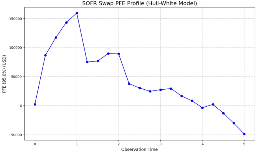

In the Real World, What Other Factors Would Be Considered When Calculating PFE?

While the Hull-White model and Monte Carlo simulation provide a strong foundation, real-world PFE calculations incorporate several additional complexities:

• Collateral Agreements (CSAs): Collateral agreements significantly reduce PFE. The PFE calculation must account for threshold amounts, minimum transfer amounts, and the frequency of collateral calls. This often involves simulating collateral flows and adjusting the exposure accordingly.
• Netting Agreements: Master netting agreements (e.g., ISDA Master Agreement) allow for the netting of exposures across multiple transactions with the same counterparty. PFE is typically calculated at the netting set level, considering all derivatives within that set.
• Wrong-Way Risk: This is the risk that exposure to a counterparty increases when the counterparty’s credit quality deteriorates. For example, if a derivative’s value increases when the counterparty’s specific industry faces economic hardship. Identifying and quantifying wrong-way risk is a significant challenge.
• Model Risk: The choice of interest rate model (e.g., Hull-White, G2++, LIBOR Market Model) and its calibration methodology can impact PFE. Understanding and quantifying model risk is important.
• Jump Diffusion Models: For certain markets, standard diffusion models might not fully capture sudden, significant market movements. Jump diffusion models can be used to incorporate these events.
• Liquidity: The ability to quickly and efficiently exit a position or re-hedge can impact real-world exposure.

Conclusion

Potential Future Exposure (PFE) is an indispensable tool for managing counterparty credit risk in derivatives trading. By providing a forward-looking, probabilistic estimate of maximum potential loss, it enables financial institutions to set appropriate credit limits, manage collateral, allocate capital effectively, and meet regulatory requirements.

While the Hull-White interest rate model, coupled with Monte Carlo simulation in QuantLib Python, offers a powerful framework for calculating PFE for SOFR swaps, real-world applications demand consideration of collateral agreements, netting, wrong-way risk, and adherence to evolving regulatory standards.

A robust PFE framework is a cornerstone of sound financial risk management, ensuring resilience against counterparty defaults in an increasingly complex derivatives landscape.

If you found this article helpful or have thoughts to share, feel free to leave a comment or reach out. I’ll be publishing more posts in this QuantLib Python series, so follow along if you’re interested in practical applications of financial engineering. Thanks for reading!

Reference

1. John C. Hull, Risk Management and Financial Institutions, 5th Edition, Wiley, 2018.
2. John C. Hull, Options, Futures, and Other Derivatives, 11th Edition, Pearson, 2022.
3. Ballabio, Luigi. Implementing QuantLib. Online resource
4. Goutham Balaraman, Luigi Ballabio. QuantLib Python Cookbook. Leanpub, 2020. https://leanpub.com/quantlibpythoncookbook
5. Damiano Brigo, Fabio Mercurio. Interest Rate Models — Theory and Practice, 2nd Edition.
6. Jon Gregory. The xVA Challenge, Counterparty Risk, Funding, Collateral, Capital and Initial Margin, 4th Edition, Wiley, 2020.