Understanding Random Noise Influence in Images Using MATLAB

How bit-level manipulation reveals the real impact of noise on grayscale images

Noise is an unavoidable phenomenon in digital multimedia — whether we are working with images, audio, or video. In digital images, noise distorts pixel values and reduces visual quality. While this topic is often discussed in terms of high-level effects, it becomes much more interesting when we analyze noise at the bit level.

This article explores how random noise affects individual bits of grayscale images and demonstrates a MATLAB implementation that visualizes this impact for each bit from LSB to MSB. The method is simple but highly illustrative, allowing us to clearly see which parts of a pixel influence its brightness the most.

🔍 Pixels, Bits, and Brightness

A grayscale pixel is represented using 8 bits, meaning its intensity can range from 0 (black) to 255 (white).

Each bit contributes differently to the final brightness:

Bit PositionWeightMeaning1 (LSB)1Very low impact22Low impact34Low impact48Noticeable impact516Medium impact632Strong impact764Very strong impact8 (MSB)128Dominant impact

The Most Significant Bit (MSB) holds half of the entire brightness range. Flipping this bit alone can darken a pixel by 128 levels — enough to dramatically change the image.

🖼️ How MATLAB Represents Grayscale Images

MATLAB loads images as matrices. For a standard 512×512 grayscale image:

• Total pixels: 512 × 512 = 262,144
• Each pixel uses 8 bits → total of 2,097,152 binary values

Internally, MATLAB stores these as arrays where pixel values range from 0 to 255. This structure makes it easy to manipulate individual bits using logical or arithmetic operations.

🎲 Generating and Applying Random Noise

In the provided implementation, noise is generated using a true random number generator based on time-dependent seed values. Unlike pseudorandom generators, this introduces a slightly more unpredictable sequence.

Noise is applied bit-by-bit, column by column:

1. Modify bit 1 (LSB)
2. Modify bit 2
3. Modify bit 3
4. …
5. Modify bit 8 (MSB)

After modifying a single bit across all pixels, a temporary image is reconstructed and displayed. This produces eight intermediate images, each showing:

• What the image looks like when only one specific bit is corrupted
• How strongly each bit contributes to visual quality

A final image is then assembled using all noisy bits combined.

📊 What the Results Reveal

The experiment makes one thing very clear:

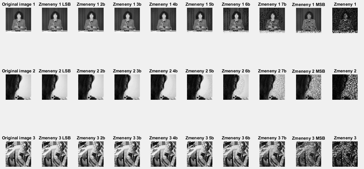
Plot by MATLAB showing noise effect on each bit separately, last image is where all bits are affected by noise (final image)

✔ Noise in MSB and upper bits drastically reduces image quality

Even minor corruption in the 7th or 8th bit results in heavy darkening or severe visual artifacts.

✔ Noise in LSB is nearly invisible

Flipping the least significant bit barely changes the image because it only affects brightness by ±1.

This makes LSB a popular target for applications like steganography, where information is hidden without noticeable visual distortion.

📈 PSNR and MSE Evaluation

The program also computes:

• MSE (Mean Squared Error) — measures how much the pixel values differ
• PSNR (Peak Signal-to-Noise Ratio) — a standard metric that expresses how noisy an image is relative to the original

Higher PSNR means better quality; lower values indicate stronger distortion. As expected:

• Images with modified MSB → very low PSNR
• Images with modified LSB → high PSNR, almost identical to original

🎨 Why Use Grayscale Instead of RGB?

Working with grayscale simplifies the demonstration:

• Only one channel instead of three
• Less memory and computation
• Easier visualization of bit impacts
• Cleaner mathematical interpretation

Using RGB would involve a 3D matrix, instead of current 2D matrix, where each pixel contains 24 bits instead of 8:

• 262,144 pixels × 24 bits = 6,291,456 binary values, so 3 times more compared to grayscale, where is was 2,097,152 binary values

The experiment is still feasible but significantly more complex — and less intuitive for teaching purposes.

📁 Test Images Used

The implementation uses three classic 512×512 grayscale images, widely used in image processing research:

• Gabriele Wohmann (lena512g.bmp)
• Noname woman (barbara512g.bmp)
• Woman image by Jamal Saeedi (girlface512g.bmp)

Each image is loaded in MATLAB using imread() and processed with identical noise patterns for consistent comparison.

lena512g.bmp

barbara512g.bmp

girlface512g.bmp

🧪 MATLAB Script

The complete MATLAB script is available here: GitHub: MATLAB-scripty / Praca_s_obrazkami / Nahodny_sum.m (https://github.com/martinius96/MATLAB-scripty/blob/main/Praca_s_obrazkami/Nahodny_sum.m)

📝 Conclusion

Bit-level manipulation provides a unique, intuitive perspective on how noise affects digital images. This MATLAB-based visualization makes it easy to see that:

• Lower bits barely influence perceived quality
• Upper bits determine the core structure of the image
• Random noise in MSB produces highly destructive distortion

This approach can be used in:

• Digital image processing education
• Error resilience studies
• Steganography experimentation
• Compression analysis
• Signal quality research

Understanding how each bit contributes to visual information is a powerful tool — especially when designing systems where noise resistance or data hiding is required.