Causal Inference 101: A Data Scientist’s Guide to Moving Beyond Correlation

Standard machine learning finds correlations to predict outcomes. Causal inference discovers the interventions that change them.

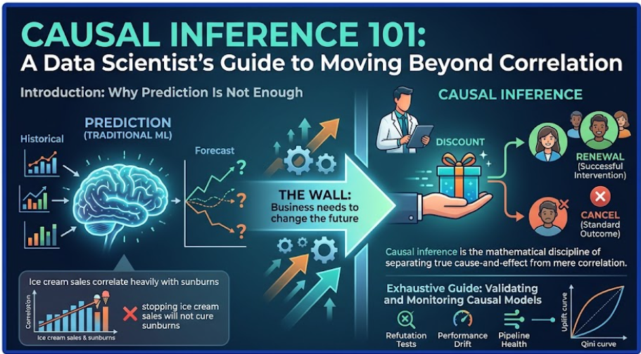
Introduction: Why Prediction Is Not Enough

Machine learning is fundamentally an engine for finding patterns. If you feed it historical data, it will find the correlations that predict future outcomes with remarkable accuracy. However, as data scientists mature in their roles, they quickly encounter a wall: the business does not just want to predict the future; it wants to change it.

Consider a classic business scenario:

• A traditional ML churn model predicts who is going to cancel their subscription.
• A causal inference model answers what action will actually prevent them from canceling.
• Sending a discount to a customer who was going to stay anyway is a waste of money.
• Sending a discount to a customer who will only stay because of the discount is a successful intervention.

Traditional algorithms cannot tell the difference between those two customers because they rely on correlation. Ice cream sales correlate heavily with sunburns, but stopping ice cream sales will not cure sunburns.

Causal inference is the mathematical discipline of separating true cause-and-effect from mere correlation. This guide covers the what, why, and how of causal inference, ending with an exhaustive look at how to validate and monitor these unique models in production.

What is Causal Inference?

At its core, causal inference is about formalizing the concept of an intervention.

To understand this, we use the Potential Outcomes Framework (often called the Rubin Causal Model). Imagine a single customer, John. We want to know the effect of sending John a 20% discount code.

• Let T be the treatment (T = 1 if he gets the discount, T = 0 if he does not).
• Let Y be the outcome (Y = 1 if he renews, Y = 0 if he cancels).

John has two “potential outcomes”:

• Y(1): What John does if he receives the discount.
• Y(0): What John does if he receives no discount.

The true causal effect of the discount on John is simply:

Individual Treatment Effect (ITE) = Y(1) — Y(0)

The Fundamental Problem

The fundamental problem of causal inference is that we can never observe both Y(1) and Y(0) for the same person at the same time. If we send John the email, we observe Y(1), but Y(0) becomes a “counterfactual” — a parallel universe we cannot see.

Because we cannot calculate the effect for an individual directly, we estimate the average effect across a population:

Average Treatment Effect (ATE) = E[ Y(1) — Y(0) ]

The Core Advantage Over Traditional ML

Why can’t we just feed a feature called received_discount into an XGBoost model and look at its feature importance?

• Confounding Variables: In the real world, treatments are rarely given randomly. Perhaps your marketing team only sends discounts to highly engaged users.
• The Bias Trap: If engaged users are already more likely to renew, your ML model will learn that received_discount is highly predictive of renewal.
• The Wrong Conclusion: The model attributes the high renewal rate to the discount, missing the fact that the underlying engagement was the true driver.

Causal inference techniques are explicitly designed to control for these “confounders” (variables that affect both the treatment and the outcome), allowing you to isolate the true incremental impact of your action.

The “How”: Basic Methods of Causal Inference

When you want to measure a causal effect, you have a toolkit of methods depending on your data.

1. Randomized Controlled Trials (A/B Testing)

• What it is: The gold standard. You randomly assign the treatment (T) to half your users and withhold it from the other half.
• Why it works: Randomization guarantees that there are no confounding variables. The treated and control groups are statistically identical, so any difference in outcome is purely caused by the treatment.

2. Propensity Score Matching (PSM)

• What it is: Used when you have observational data (non-randomized). You train a model to predict the probability of a user receiving the treatment (their propensity score).
• How it works: You take a treated user and find an untreated user with the exact same propensity score. By matching them, you create an artificial “control group” that looks just like your treated group, mimicking an A/B test.

3. Difference-in-Differences (DiD)

• What it is: A technique used when a treatment is applied to one entire group (e.g., a specific city) but not another, over a specific point in time.
• The Formula: DiD = (Y_T,post — Y_T,pre) — (Y_C,post — Y_C,pre)
• How it works: You measure the change in the treatment group before and after the intervention, and subtract the baseline change in the control group. This accounts for natural time-based trends.

4. Instrumental Variables (IV)

• What it is: Used when there is unmeasured confounding. You find a rare variable (the instrument) that affects the treatment but has no direct effect on the outcome.
• Example: If you want to measure the effect of a new app feature (treatment) on retention (outcome), but feature adoption is driven by user motivation (unobserved confounder), you might use “being assigned to a specific server” (instrument) that makes the feature load faster.

Exhaustive Guide: Validating and Monitoring Causal Models

If you build a standard predictive model, you can monitor its accuracy in production by comparing predictions to actual outcomes.

Causal models are different. Because you never observe the counterfactual (Y(0)), you can never definitively say if your causal estimate for a specific person was right or wrong. Therefore, monitoring and validating causal models requires a specialized, exhaustive approach spanning three distinct layers: Refutation, Performance Drift, and Pipeline Health.

Layer 1: Pre-Deployment Refutation Tests

Before you ever trust a causal model, you must try to break it. Refutation tests check if your model is capturing true causality or just complex noise.

• Placebo Treatment Test: Replace your actual treatment variable with a randomly generated dummy variable, then rerun your causal model. If your model detects a significant causal effect from a random variable, your methodology is flawed. The effect should drop to zero.
• Dummy Outcome Test: Replace your actual target metric with a variable you know cannot be affected by the treatment (e.g., user behavior before the treatment occurred). The estimated effect must be zero.
• Subset Removal Test: Randomly drop 10% to 20% of your data and re-estimate the causal effect. A robust causal model should yield a stable Average Treatment Effect (ATE). If the estimate swings wildly, your model is overly sensitive to outliers.
• Unobserved Confounder Addition: Simulate a fake, unobserved confounding variable and inject it into your dataset. If a minor unobserved confounder completely changes your estimated effect, your model is fragile.

Layer 2: Post-Deployment Causal Monitoring

Once your model (often deployed as an Uplift Model) is in production, you must monitor its ongoing validity.

• Continuous Global Holdouts: This is the most critical monitoring tool. Always keep a small, randomized 2–5% holdout group that receives the standard baseline treatment. By continuously comparing your causal model’s targeted group against this holdout, you can measure the true, ongoing cumulative lift.
• Qini Curve and Uplift Curve Tracking: Uplift models output a score representing the expected causal impact. In production, you group users by deciles based on this score and monitor their actual behavior. If the top decile (predicted highest impact) stops outperforming the bottom deciles, your model’s causal validity has degraded.
• Treatment Effect Drift: Track your estimated ATE over time. If your intervention (e.g., a discount) historically yielded a +5% lift, but begins trending toward +1%, the market has adapted to your intervention. The causal mechanism has shifted, and the model requires retraining.

Layer 3: Causal Covariate and Pipeline Monitoring

Causal models are highly sensitive to the distribution of their input data. If the underlying population changes, your causal estimates are no longer valid.

• Population Stability Index (PSI): Monitor the PSI for all confounders used in your model.
• Formula: PSI = Σ (Actual% — Expected%) × ln(Actual% / Expected%)
• If PSI > 0.25 on a key confounding variable, the population has shifted significantly, meaning your artificial control groups (like in PSM) are no longer balanced.
• Propensity Score Distribution Drift: For matching methods, track the distribution of the propensity scores. If the overlap between the treatment and control score distributions shrinks over time, it indicates that treatment assignment in the real world has become highly deterministic, making causal estimation impossible.
• Data Pipeline Freshness and Null Rates: A causal model relies on precise timing (cause must precede effect). Monitor pipeline freshness to ensure features are not delayed. Track null rates rigorously; missing data in a confounder can instantly break the conditional independence assumption your model relies on.

Conclusion

Causal inference requires a shift in mindset. You are no longer just fitting a curve to data; you are attempting to uncover the hidden rules of how one action influences another.

While the mathematics can be challenging, the business value is immense. A data scientist who understands causal inference stops telling the business what will happen, and starts telling the business how to change what will happen. By pairing these methods with rigorous, exhaustive refutation and monitoring practices, you can build systems that drive verifiable, incremental value.