I Tried to Put a Diffusion Model on a Mac. NumPy Had Other Plans.

[Error: Only 0-dimensional arrays can be converted to Python scalars: exporting SDXL to Core ML in 2026]

This is less a project write-up than a record of everything that broke on the way. That turns out to be the useful part.

This project started with a simple, slightly greedy wish. I wanted a full image generator the kind that paints a picture from a sentence, running inside a Mac. No server. No cloud. No spinner.

But there was a second reason, and it’s the honest one.

Training a model and serving a model are two different disciplines that happen to share a vocabulary. Training is about loss curves, data, architecture while Serving is about everything after that does it fit, does it fit in memory, how many milliseconds, on what hardware, in what numeric precision, and does the compiled artifact still produce the same numbers as the thing you trained?

Almost nobody talks about the second half, and it’s where most models quietly die between a working notebook and something a person can actually use. That second world is the one I’m drawn to. This project was me deliberately walking into it

I got there. But the interesting part isn’t the demo, it’s the two days I spent trapped between two libraries that refused to be in the same room.

Let me walk you through it.

Part 1: Making it fast

I started with SSD-1B, a distilled variant of Stable Diffusion XL. Good images, roughly half the parameters of full SDXL.

If you haven’t looked closely at how these things work, the mechanism is worth a paragraph, because everything that goes wrong later comes straight out of it.

A diffusion model doesn’t paint. It un-destroys. During training you take a real image, add a controlled amount of random noise, and ask the model a single question: what noise did I just add? Do that across millions of images and every noise level, and the model becomes very good at looking at a mess and identifying which part of it is garbage. Then you flip it around at generation time. Start with nothing but pure noise, ask the model what’s garbage, subtract a bit of it, and ask again. Repeat, and an image that was never there emerges out of the pure noise

The component doing that guessing is the UNet, and it’s the heavyweight of the pipeline the billion parameters, and effectively all the compute. It’s called a UNet because of its shape it squeezes the image down through a series of blocks into a small, dense representation, then expands it back up. On the way down and back up sit the cross-attention layers, which are where your prompt actually gets in.

Two other pieces travel with it. The text encoder turns your prompt into vectors the UNet can attend over. And the VAE is a compressor that makes computation lot more easier: rather than denoising a full 1024×1024 image, everything happens in a smaller latent space, and the VAE decodes that latent back into real pixels only at the very end. A 1024×1024 RGB image is about 3.1 million values. Its latent is 128×128×4 around 65,000. That’s roughly 48× less data.

So the pipeline is: prompt → text encoder → many UNet passes in latent space → VAE decode → image.

And there’s the problem. It’s not that the UNet is big. It’s that it runs thirty to fifty times per image. On an A100 that’s fine. On a Mac, fifty passes through a billion-parameter UNet is a coffee break, and the UNet is where I’d be spending all my optimization effort for the rest of the project.

So the first move was converting it into a Latent Consistency Model. Here’s the idea. A normal diffusion model is stubbornly incremental. It only knows how to get from noise to slightly less noise, so to reach a finished image it has to make that same small move over and over, fifty times. It can never see more than one step ahead it’s working the problem line by line down the page. An LCM learns the whole trajectory as a single function. Instead of walking the path, it maps the starting noise directly to where that path ends. It’s the Ramanujan version of the same model: everyone else is grinding through the working, and this one reads the question and writes down the answer.

(In practice you still take about four steps rather than one. A couple of refinement passes buy back most of the fine detail you lose by jumping. But four instead of fifty is the difference that is needed for optimization)

The part I find genuinely elegant is how cheap this transformation is. You don’t retrain the model retraining SSD-1B from scratch is not a thing that happens on my desk. Instead you use a LoRA: a small set of low-rank adapter matrices that sit alongside the frozen original weights and nudge their behavior by adding some values to the original weights. The base model doesn’t move. You only ever train that tiny delta, and in my case I didn’t even do that someone already published it.

Then you fuse the delta into the weights, and the model simply is an LCM now. Same architecture, same parameter count, completely different behaviour. You didn’t send it back to school; you handed it a technique.

One more thing has to change alongside it. The scheduler is the component that decides how much noise to remove at each step, and the default one assumes the slow incremental walk. Swap in LCMScheduler.

You go 50 → 4 steps, you also go 2 → 1 UNet calls per step. That’s a ~25× reduction in forward passes before you’ve compressed anything at all.

Fast. Still too big.

Part 2: Making it small (palettization, not quantization)

People hear “compression” and think quantization. Palettization is its close cousin, but the mechanism is different and the difference matters.

Quantization takes a float16 weight and maps it onto a smaller numeric grid typically int8 using a scale.

Palettization doesn’t round. It runs k-means over the weight tensor, finds a small set of representative value the palette, or lookup table and replaces every weight with a tiny index pointing into that table. 6-bit palettization means 64 distinct values survive per group.

The photo analogy is exact: it’s the difference between dimming a photo (quantization) and reducing it to a 64-colour GIF (palettization). And it’s the format Apple’s Neural Engine is happiest with.

I used SKMPalettizer (Sensitive K-Means) plain k-means treats every weight as equally important, which is nonsense; some blocks of a UNet carry far more signal than others. SKM weights the clustering, so it spends its precision budget where the model actually cares.

That compute_sensitivity call took about six hours on my Mac, which is why the very next thing I wrote was a cache. Do not learn this the hard way like I did.

The W6/W8 split wasn’t a guess, I ran a per-block sensitivity sweep first and let the FID/CLIP numbers decide which blocks got the extra two bits.

Part 3: What “converting to Core ML” actually means

This phrase gets thrown around like it’s one button. It’s actually a chain of four artifacts, and each hand-off is a place things can break.

Step zero: save the PyTorch model. After palettization, the compressed pipeline gets written to disk in diffusers format which is a directory of config.json and .safetensors files.

pipe.unet = compressed_unet
pipe.save_pretrained("file/to/local/directory")

Step one: trace it. Reload that saved model, and now convert it from Python into something static. Your model is PyTorch which is a graph of tensor operations expressed as Python. A phone cannot run Python. So you push one representative example through the model and record every operation it performs, in order. You’re watching someone cook once and writing down the recipe.

torch.jit.trace is what does this

traced = torch.jit.trace(wrapper, example_inputs)
traced.save("Output/path/") 

This is saved as .pt file, that .pt file is a self-contained, Python-free description of the UNet. Being able to save it separately is genuinely useful during debugging, when conversion blows up at operation 313 for the fifth time, you want to reload the trace in two seconds rather than rebuild the whole pipeline.

The catch with tracing is that it records exactly one path. Any if statement branching on a tensor value gets frozen to whichever branch your example happened to take, and any dynamic shape gets baked in as a constant.

And there’s no way around it. This is the first real trade off I encountered for serving the model locally. It’s worth knowing exactly what you gave up, though.

Your model is now one resolution, forever.

Remember the model doesn’t work on pixels, it works on the latent space (compressed space). The VAE shrinks by a factor of 8 in each direction, so a 1024×1024 image becomes a 128×128 latent. That’s the (2,4,128) I traced with:

• 2 is two images at a time
• 4 is the latent has 4 channels (a normal image has 3: red, green, blue)
• 128 × 128 is the height and width of the latent, which is 1024 ÷ 8

Now, in ordinary PyTorch, this would never be a problem. Write a model in normal Python, feed it a 1024 image, it computes 128, feed it a 512, it computes 64.

Tracing asks that question once, gets the answer 128, and writes 128 down permanently.

The model is now a fixed number. Hand it a 512×512 image, the latent arrives at 64×64, and a few hundred operations downstream are still confidently expecting 128. It doesn’t adjust. It just breaks.

And you do want other resolutions in real life. A few obvious cases:

• Previews. Generate a quick 512×512 draft in a second so the user can see whether they like the composition, then run the full 1024 only when they commit. Nobody wants to wait for a full-quality render of an image they’re about to discard.
• Shape. A phone wallpaper is tall, not square. A profile picture is small and square. 1024×1024 is one shape and real apps need several.
• Older phones. A device with less memory might only survive 512×512. Right now I have nothing to offer it.

So if I want 512×512 as well, there’s no clever fix. I trace again with a 64×64 latent.

Two things that cost me real time during Python to Apple Conversion

1. The prompt tensor has to be three-dimensional

encoder_hidden_states is your prompt after the text encoder has turned it into numbers. Its shape is (2, 77, 2048):

• 2 is two prompts at once
• 77 is word-slots. CLIP always pads to 77, so a three-word prompt and a forty-word prompt both arrive as 77 slots.
• 2048 is numbers describing each slot. SDXL uses two text encoders, 768 + 1280.

Three numbers means three dimensions.

I fed it in as four dimensions instead: (2, 2048, 1, 77).

That was deliberate. The Neural Engine is built around 4D tensors, and Apple’s own reference implementation transposes the prompt into that shape so I matched it, hoping for the faster path on-device.

But diffusers’ UNet doesn’t understand that layout. It wants rank-3. So the model took rank-4 at the door and my wrapper transposed it straight back to rank-3 before handing it to the UNet: this is forced by tracing. Because the graph is static, whatever shape I declare at the boundary is the shape the model accepts forever.So, if I want the ANE-friendly rank-4 as the public input, the conversion back to rank-3 has to happen inside the traced graph itself. There’s nowhere else to put it.

The UNet’s one job is to look at a noisy image and predict the noise in it. So how do you check whether a prediction is any good? You don’t need the right answer you can just measure how strong the prediction is.

Here’s why that works.

The prediction isn’t one number it’s a grid of about 131,000 of them, one for every position in the latent (2 × 4 × 128 × 128). Each one is the model’s guess for how much noise is sitting at that spot, and each can be positive or negative.

Now, where did the real noise come from in the first place? torch.randn. That draws from a standard normal distribution, which is defined by two properties: the values average out to 0, and their standard deviation is exactly 1.0. In practice that means most of the numbers land between −1 and +1, a few stray out to ±2 or ±3, and they're symmetric around zero.

Standard deviation is just the typical distance of a value from the average. Spread of 0.2 means everything is huddled tightly around zero. Spread of 1.0 means values are routinely a full unit away in either direction.

So the check is: take all 131,000 predicted numbers, compute their standard deviation, and see whether it’s near 1.0 because that’s the character of the thing the model was trained to reproduce.

PyTorch gave me 0.98. Textbook.

Core ML gave me 0.58.

And the useful part is that 1.0 is the expected answer at every step. The amount of noise sitting in the image changes enormously as you proceed, scaling is the scheduler’s job, handled separately. The UNet itself is always predicting the same normalized quantity. So there’s one fixed number to check against, at any point in the process, which makes this a cheap and reliable test.

Same input, same weights, and the prediction came out at roughly 60% strength. The model was still pointing in the right direction it just wasn’t saying it loudly enough.

And that’s fatal. The error compounds and the final image was only noise. It doesn’t look like a bug, it looks like a model that doesn’t work.

So the problem was never the model or the weights. It was the layout conversion I’d asked Core ML to perform on the incoming prompt.

The fix was to stop asking. Don’t take rank 4 at the door and convert it inside the graph just take rank-3 directly.

So what did I lose by dropping Apple’s layout?

The rank-4 channels-first arrangement isn’t a requirement of the Neural Engine it’s an optimization for it. Core ML happily compiles and runs a rank-3 model, and the ANE will still take most of the work. What you give up is the smoothest path: the ANE is built around 4D tensors, so with rank-3 the compiler may insert its own reshapes internally, or hand a few operations to the GPU instead. This is the second tradeoff I gave up for conversion I traded efficiency for consistency

2. The time step has to be a decimal

The time step is just a number telling the UNet which stage of denoising it’s on. The UNet needs it because “how much of this is noise” depends entirely on where you are.

The bug was boring. PyTorch gives you 999. Core ML wanted 999.0. Same value, different type, and the converter won't bridge it for you. One character.

But here’s the cruel part. That bug crashed with the exact same error message as the NumPy problem in the next section

only 0-dimensional arrays can be converted to Python scalars

So I fixed the dtype, re-ran, saw an identical error in an identical place, and concluded my fix hadn’t worked. It had. A completely unrelated bug was waiting directly behind it.

Here’s what tracing actually looks like when you run it, and it is not reassuring:

…/diffusers/models/upsampling.py:147: TracerWarning: Converting a tensor to a
Python boolean might cause the trace to be incorrect. We can't record the data
flow of Python values, so this value will be treated as a constant in the future.
This means that the trace might not generalize to other inputs!
 assert hidden_states.shape[1] == self.channels
…/diffusers/models/upsampling.py:162: TracerWarning: Converting a tensor to a
Python boolean might cause the trace to be incorrect. …
 if hidden_states.shape[0] >= 64:

Dozens of these scroll past. And here’s the thingmost of them genuinely are harmless, which is exactly what makes them dangerous. You get trained to scroll past a wall of yellow, and then the one warning that did matter goes past with the rest. Read them once, properly, the first time.

Step two: conversion. coremltools walks that traced graph and rewrites each one into Apple’s intermediate language, MIL.

import coremltools as ct
import numpy as np
mlmodel = ct.convert(
 traced,
 convert_to="mlprogram",
 inputs=[
 ct.TensorType(name="sample", shape=(2, 4, 128, 128), dtype=np.float16),
 ct.TensorType(name="timestep", shape=(2,), dtype=np.float16),
 ct.TensorType(name="encoder_hidden_states", shape=(2, 77, 2048), dtype=np.float16),
 ct.TensorType(name="text_embeds", shape=(2, 1280), dtype=np.float16),
 ct.TensorType(name="time_ids", shape=(2, 6), dtype=np.float16),
 ],
 outputs=[ct.TensorType(name="noise_pred", dtype=np.float16)],
 compute_precision=ct.precision.FLOAT16,
 minimum_deployment_target=ct.target.iOS18,
 compute_units=ct.ComputeUnit.CPU_AND_NE,
)

Step three: save and compile.

mlmodel.save("UNet.mlpackage")

An .**mlpackage** is a directory, not a file. Xcode compiles it into an .**mlmodelc** at build time. You can do that yourself too:

xcrun coremlcompiler compile UNet.mlpackage ./compiled/

So the full arc: **PyTorch → traced graph → MIL → .mlpackage → .mlmodelc → Neural Engine.**

**Part 4: The dinner party from hell**

You watch the progress bar crawl, and then it just stops:

Converting to CoreML mlprogram… Converting PyTorch Frontend ==> MIL Ops: 9%|███▊ | 313/3464 [00:00<00:00, 5702.10 ops/s] Saving value type of int64 into a builtin type of int32, might lose precision!

And then:

File "…/coremltools/converters/mil/frontend/torch/ops.py", line 3048, in _cast res = mb.const(val=dtype(x.val), name=node.name) TypeError: only 0-dimensional arrays can be converted to Python scalars

Which is, roughly, the software equivalent of your car refusing to start and the dashboard simply displaying the word *no*.

Here’s what’s actually happening. NumPy used to be accommodating: if you had a size-1 array and asked for it as a plain Python number, it would quietly hand it over. NumPy 2.4 removed that. You now have to call `.item()` explicitly.

coremltools 9.0’s Torch frontend was written against the old, friendly behaviour. So when it hit a shape-arithmetic constant mid-conversion and called **int()** on it the casual way, NumPy 2.4 refused.

It’s a known issue — [apple/coremltools #2633]([https://github.com/apple/coremltools/issues/2633](https://github.com/apple/coremltools/issues/2633)), filed December 2025. Not my discovery. I just rediscovered it the slow way.

And the documented fix is one line:

pip install "numpy<2.4"

Which works. And then immediately breaks something else:

ImportError: cannot import name 'NP_SUPPORTED_MODULES' from 'torch._dynamo.utils'

Downgrade NumPy, while having torch 2.11 is that you don’t lose a feature, you lose `torch._dynamo` entirely.

So: coremltools demands NumPy < 2.4. torch 2.11 demands NumPy ≥ 2.4. There is no version of NumPy that satisfies both. This is the part that isn’t in the issue thread, and it’s the part that actually cost me the day.

**Part 5: Two rooms**

The fix is not a magic version. There isn’t one. The fix is accepting that these two jobs don’t have to happen in the same place.

Training, LoRA merging, sensitivity analysis, evaluation that all stayed in my main environment on modern versions. Then I built a second, sealed environment whose only job in life is to run the export:

python3.12 -m venv .coreml-export source .coreml-export/bin/activate pip install \ torch==2.7.0 \ torchvision==0.22.0 \ transformers==4.46.3 \ diffusers==0.31.0 \ "accelerate>=1.0,<1.5" \ "numpy>=2.0,<2.4" \ coremltools==9.0

torch 2.7 doesn’t need NumPy 2.4. Nobody in that room is fighting. The workflow becomes: do the model work in the main environment, save the compressed pipeline to disk, step into the sealed one, run the conversion, step back out.

The lesson I’d actually hand to someone else: when two dependencies pull in opposite directions, stop looking for the version that makes everyone happy. Sometimes the right answer is two rooms and a hand-off through the filesystem.

**Part 6: Did it work?**

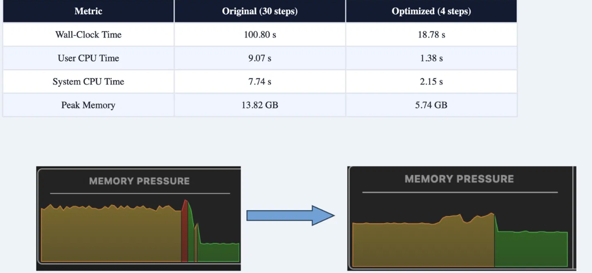
Yes, eventually. 5.4× faster, 2.4× less memory. The UNet went from 2,539 MB at FP16 down to 1,272 MB as a Core ML package, and the full bundle landed at roughly 2.9 GB.

![](https://miro.medium.com/v2/resize:fit:1188/1*HVOozpKP3t3H_h-X9iwW2w.png)