Media Mix Modeling: Too Many Parameters, Too Little Data

I have a little confession to make: I am a bit envious of my product analytics colleagues. They get to work with A/B tests, the gold standard of causal inference with clean counterfactuals, huge sample sizes, and parameters that are well behaved. Meanwhile, in the marketing science pit, we are knee-deep in observational data, trying to extract causality from a chaotic mixture of covarying spend patterns, promotional events, seasonality, competitor actions, macro factors and noise. You know, the usual Tuesday where seasonal campaign spend, Valentine’s Day promotions, and a competitor’s price cut all happened in the same week.

But we keep trying anyway, because marketers need to know whether their campaign worked, and if so, how much. With multi-touch attribution gone, Media Mix Modeling (MMM) has come roaring back. There are now many open-source libraries out there, like Facebook’s Robyn, Google’s Meridian, and PyMC-Marketing by PyMC Labs. But the resurgence hides an uncomfortable truth:

Modern MMM often has more parameters than information to estimate them.

Let’s talk about why.

Do you want to build a sandwich?

On paper, the core idea of MMM is fairly straightforward:

1. You have a KPI time series. It goes up and down. Cute.
2. Take your media spend time-series, transform them by applying adstock (the lagged effects of an ad) and saturation functions of your choice
3. Stack the transformed signals and regress them against the KPI.

It’s basically a line fitting optimization problem. How hard can it be?

Very, as it turns out.

These transformations are nonlinear, correlated, and lagged, which results in a problem called non-identifiability. This means that you can have a set of solutions that give you really good, equally optimal fit but no way to tell which one is truer based on the data.

To illustrate this, imagine you’re an alien who has never been to Earth. Your friend, who just finished a vacation there (“it’s beautiful this time of the year!”), told you about this wonderful human delicacy called the BLT: the glorious bacon-lettuce-tomato sandwich. You are intrigued, so of course you go to your alien artificer wonder machine to try to replicate it. You have learned from your friend that this BLT sandwich has

• Total weight of 200g
• Made of toast, bacon, lettuce, tomato, and mayonnaise

… but that’s all you know. Your friend didn’t tell you anything else. Now, with this information, can you make a sandwich?

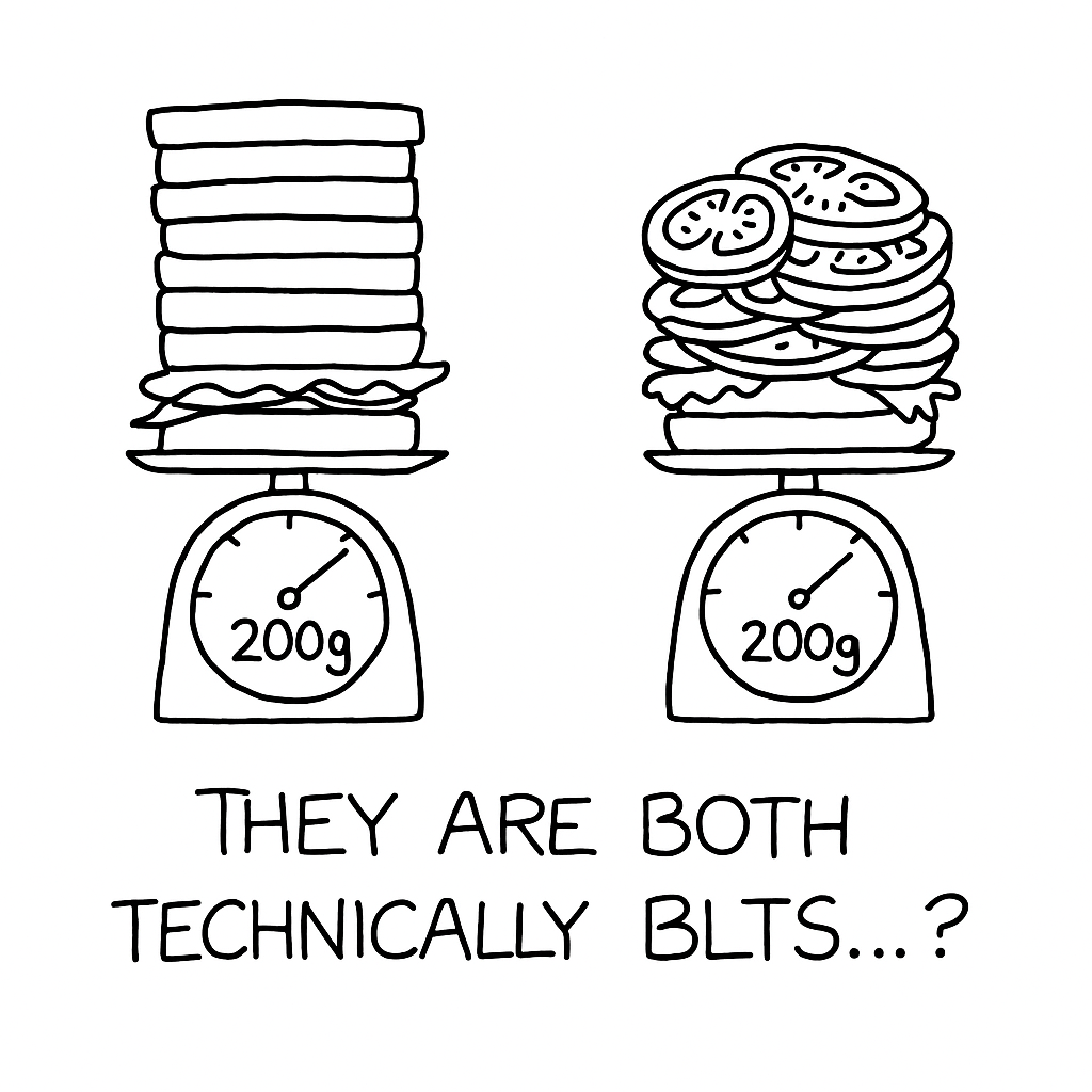
Well, unfortunately no. With these constraints you can end up with sandwiches that are 140g toast, 10g rest of the ingredients and still satisfies the conditions.

To get anywhere close to a sane sandwich you will need more information, for example an approximate ratio of lettuce, tomatoes, bacons, etc. This is MMM’s problem in a nutshell. The KPI is the sandwich weight, and the distribution of media effects is potentially unknowable. Just as there are infinite ways to distribute 200g across sandwich ingredients, there are infinite ways to distribute KPI lift across correlated media channels that all ramped up together during the holiday season.

Multiple parameterizations can fit the same KPI equally well. Despite identical goodness-of-fit metrics (RMSE), each model attributes the KPI lift very differently across channels. This is the core non-identifiability problem in Media Mix Modeling.

You might think, “okay, so the model can’t perfectly separate effects. But if the total is right, isn’t that good enough?” Not quite. The whole point of MMM is to inform budget allocation decisions: which channels deserve more spend, which should be cut? If the model says “Facebook drove 40% of lift, and Instagram drove 20%” but it could just as easily be “Instagram drove 40%, Facebook drove 20%” with the same fit quality. You’re making million-dollar decisions on a coin flip.

This is where modern MMM frameworks step in with different philosophies on how to break the tie.

Robyn and Meridian — Different Approaches to the Same Problem

What is needed to break out of the non-identifiability zone and into something resembling a robust model is additional information: what you already kind of know, something that can help you restrict the plausible range of the parameter values.

Looking at it this way, we can see that encoding additional information into the model fitting process is practically required when dealing with large number of parameters. Robyn and Meridian are two different MMM implementations that try to solve the same problem with its own way of encoding prior information.

Robyn: Multi-objective survival

Robyn tackles identifiability through multiple objective functions: fit, realistic spend/effect distribution (DECOMP.RSSD), and calibration alignment. The model that gets selected need to be Pareto optimal, i.e. good model by all criteria. It’s essentially semi-Bayesian, with priors expressed indirectly through calibration constraints and regularization penalties.

Meridian: Full Bayesian Uncertainty

Meridian takes on the uncertainty more directly with a Bayesian approach. You encode your pre-modeling information in the form of priors, and the MCMC sampling algorithm explores the parameter space to produce posterior distributions based on your priors and the data. The resulting posterior distributions show you the range of plausible parameter values. Wide posteriors reflect true ambiguity in the data, while narrow posteriors indicate the data was informative. Where data is weak, priors exert stronger pull on the final estimates.

Some of you might be wondering, “well jeez, I’m doing MMM because I don’t know about the media contribution of the channel I want to know about,” which is true and fair. To be frank, these prior information come from a messy intersection of platform characteristics, historical learnings, geo-lift experiments, domain knowledge, cross-functional context, and modeling judgment. And this is exactly the point: building effective MMM is less of a precise science and more of an art of systematically integrating what you do know.

MMM as Part of an Triangulation System

Here is the most important shift in mindset most marketers need to have about MMM: it’s not a ground truth generator, where you input your historical data and out comes a clean estimation of how much the marketing channels contribute to your KPI. MMM acts best when it’s used as an integrator of information that systematically incorporates what you know, and how confidently, about your marketing campaigns.

This is why our analytics team here at Pairs, and Match Group in general, are moving towards a triangulation approach where we use multiple sources of information to help pin-point the estimate:

1. Fast-moving OrbitML based Bayesian Structural Time Series

We use BSTS models to quickly capture channel efficiency signals on a rolling basis. The “fast-moving” part is key. These models update weekly and can detect shifts in channel performance much faster than traditional MMM refresh cycles. Bayesian structural time series naturally decompose the KPI into trend, seasonality, and channel effects using state-space models, giving us a baseline understanding of what’s driving changes week-to-week.

2. Selective geo-holdout tests

For high-stake, high-ambiguity channels, for example a new upper-funnel TV campaign where we genuinely don’t know if it works, we run geo-holdout experiments. We hold back spend in randomly selected markets and measure the difference. This gives us quasi-experimental, causally credible estimates that become strong priors in the MMM. For example, if a geo-test shows YouTube brand campaigns deliver a 1.5x-2.0x ROAS, we can encode this as a prior distribution in the MMM model.

3. Last-touch attribution and platform metrics

While last-touch attribution has well-known biases (it over-credits lower-funnel channels), it still provides a useful supplemental signal. We don’t, and shouldn’t, treat platform-reported conversions as ground truth, but we do use them as loose upper or lower bounds. If Google Ads reports 1000 conversions and MMM allocates 50, something is probably wrong.

4. MMM with integrated priors

Finally, we run the full MMM model with learnings from steps 1–3 encoded as priors. The OrbitML estimates inform our expectations for baseline channel efficiency. The geo-test results become tight priors on specific channels. The attribution metrics serve as soft calibration targets. The MMM then produces a holistic view that respects all these partial truths while maintaining internal consistency about how channels interact (saturation, adstock, synergies).

This way, MMM isn’t treated as oracle (which it cannot be), but a model that weaves together all partial truths.

Final Thoughts

Marketing effectiveness will never be perfectly knowable. User journeys and how our marketing touch points interact with them are highly complex and non-linear. It is no wonder that even with modeling technique as sophisticated as MMM, historical data alone will never give you the guaranteed truth. But utilized wisely, MMM can be a powerful platform to integrate all the loose information you have about your marketing campaigns.

You may never get the perfect BLT sandwich, but at least it won’t be 90% toast.