DuckDB: The Death Of Small-Scale Spark

While everyone debates the future of distributed compute, a single binary is quietly replacing Spark clusters for most of the data pipelines in most of the stacks you will actually encounter.

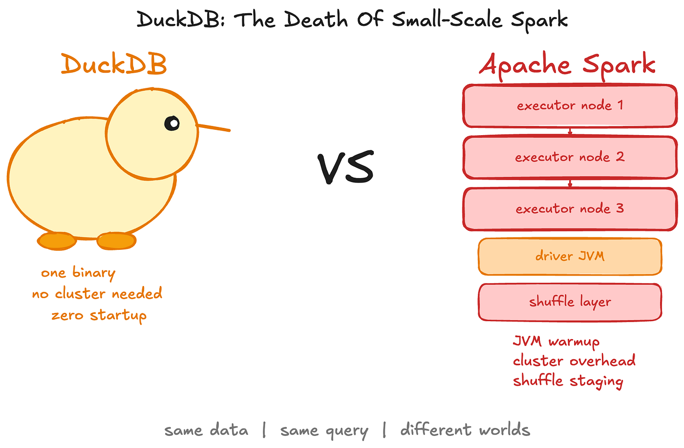
There is a Spark job running somewhere right now on a managed cluster. It reads 8 GB of Parquet, runs three aggregations, and writes a result table. The whole thing takes four minutes. Two of those minutes are executor negotiation, JVM warmup, and shuffle staging. The actual computation takes under thirty seconds.

Nobody questions it. The cluster was already there. Spark was the standard. So the pipeline stays.

This is a story about that decision, and the cost of never revisiting it.

The Reflex That Is Costing You Time

Data engineers learn Spark early and apply it everywhere. The mental model locks in fast: large data requires distributed compute, and distributed compute means Spark. That logic was sound for a long time. It is eroding now, and the erosion is measurable.

The question worth asking before any new pipeline is not “how do I run this on Spark?” The right question is “does this job actually need a cluster?”

For most pipelines processing under 50 GB on a single developer machine, the honest answer is no. The cluster adds JVM overhead, executor spin-up latency, shuffle staging cost, and configuration complexity to a problem that a single binary could finish in seconds. The engineer pays the distributed tax without receiving the distributed benefit.

The threshold is not a fixed law. A 16 GB laptop hits memory pressure around 20 GB of data. A 128 GB VM with NVMe scratch space handles well past 100 GB. The number depends on your machine. The principle does not.

This article is about two things. First, the concrete evidence that DuckDB outperforms Spark on small and medium data by a significant margin. Second, the practical setup to run your own pipelines, including a working ETL from Parquet through to an Iceberg lakehouse, using a single Python process and no cluster.

It is also honest about where Spark wins. Because it does.

Why DuckDB Is Structurally Faster On One Machine

Before the benchmarks, the mental model matters. Speed claims without mechanism are just marketing.

DuckDB is not a server. It is not a framework. It is a library. It runs inside your Python process, your R session, or your command line. There is no TCP connection between your code and the query engine, no result serialization, no driver protocol overhead. The engine lives in the same memory space as your script, which eliminates an entire category of latency that distributed systems carry as a permanent structural cost.

The diagram below shows exactly where the cost difference lives.

In-process versus cluster execution model across the full stack from query entry point to storage.

On the DuckDB side, there are no moving parts to start before computation begins. On the Spark side, there are several.

The Engine Itself

DuckDB processes data in columnar batches called vectors, roughly 1,024 rows at a time. Each vector is sized to maximize CPU cache utilization, which lets the processor use SIMD instructions to operate on entire columns at once instead of row by row. Vectorized execution dramatically improves cache locality and reduces memory-access overhead compared with row-at-a-time models.

Thread management follows a morsel-driven model. Each thread takes its own segment of input and maintains its own local hash table or sorted run, with no lock contention during the compute phase. The combine step runs across all cores after each thread finishes. The result is full CPU utilization with near-zero coordination overhead.

When data exceeds available RAM, DuckDB’s buffer manager spills to disk adaptively. Grouping, sorting, joining, and windowing all support out-of-core execution. Hannes Mühleisen demonstrated this live at PyData Amsterdam 2025: a 265 GB dataset with 6 billion rows, running COUNT DISTINCT, completed in 46 seconds using only 2 GB of memory.

No cluster required. No executors to negotiate. Startup overhead is typically negligible compared with Spark, where executor negotiation alone adds tens of seconds to minutes on managed clusters.

The key insight is this: DuckDB’s in-process design does not just remove infrastructure complexity. It removes entire categories of latency that Spark treats as the cost of doing business at scale. For workloads that fit one machine, that cost is pure waste.

The Benchmark Evidence

Claims without data are opinion. Here are the numbers, with named sources and methodology.

The table below summarizes four independent tests across a range of scales and workload types.

Wall-clock time, peak memory, and CPU behavior across four independent tests ranging from 23 GB to 1 TB.

The Laptop Test: Up To 100x On Sub-20 GB

Matt Martin and Zach Wilson at DataExpert.io benchmarked DuckDB against vanilla Spark on a 16 GB RAM laptop across seven synthetic Parquet datasets up to 23 GB. The workload was COUNT DISTINCT on a random string column, designed to force full file scans with no optimization shortcuts. DuckDB was faster in every single run, including the 23 GB dataset that exceeded the machine’s RAM. Their published conclusion: on the tested COUNT DISTINCT workloads, DuckDB was up to roughly 100 times faster than Apache Spark on sub-20 GB datasets.

Matt’s working rule from that benchmark: default to DuckDB, switch to Spark when data exceeds approximately 20 GB on a 16 GB machine. Not a hard data limit. A memory pressure threshold.

The Production Pipeline: Measured With perf stat

Digital Turbine’s engineering team ran a more rigorous test in March 2025, using Linux perf stat to capture CPU behavior, not just wall-clock time. The workload was a group-by aggregation on 40 GiB of Parquet across 52 files and 94 columns, on a 16-core, 64 GB cloud VM.

DuckDB finished in 3.99 seconds. Spark took 16.39 seconds. The memory and CPU numbers tell a sharper story than the 2.5x speed gap alone. DuckDB consumed 196 MB of peak RSS. Spark consumed 1.65 GB. DuckDB triggered 6,726 context switches and 130 CPU migrations. Spark triggered 185,639 context switches and 16,303 CPU migrations.

Those numbers are JVM warmup, garbage collection, and a distribution-oriented execution plan imposing real cost on a job that never needed distribution. Digital Turbine replaced this pipeline with a DuckDB Kubernetes CronJob. The Spark version was a 100-line Scala project with an sbt build. The DuckDB replacement was six lines of Python and a pip install.

The Honest Ceiling: Where Spark Wins Back

Miles Cole’s LakeBench study on Microsoft Fabric, published in June 2025 and fully open-sourced, is the most rigorous independent test and the most important for calibrating expectations.

At 140 MB and 1.2 GB compressed, single-node engines beat Spark cleanly. At 12.7 GB, Spark with a Native Execution Engine was fastest, with DuckDB competitive. At 127 GB compressed, Spark ran 3.5 to 6 times faster than DuckDB depending on core count. DuckDB ran out of memory at 16 cores on that test.

The cost dimension from endjin’s parallel Fabric study adds context: the cheapest Spark run costs more than five times the cheapest DuckDB run, even at scales where Spark wins on wall-clock time. Speed and cost are separate questions, and they sometimes have different answers.

The evidence points to a clear threshold. Below roughly 50 GB on a standard developer machine, DuckDB wins on speed, cost, and operational simplicity. Above 100 GB compressed, Spark with a native vectorized engine pulls ahead on speed, though at significantly higher infrastructure cost. Between those two points, you should benchmark on your actual data.

Setting Up Your Environment In VS Code

The setup takes under five minutes. That fact is itself an argument.

Install With uv

uv is the current default Python package manager for engineers who care about speed and reproducibility. Install it once, then initialize a project:

# Install uv if you do not have it
curl -LsSf https://astral.sh/uv/install.sh | sh

# Create the project
uv init duckdb-pipeline
cd duckdb-pipeline

# Add dependencies
uv add duckdb pandas pyarrow

# Run any script with the managed environment
uv run any_script.py

No JVM. No cluster configuration. No executor memory tuning. DuckDB is approximately 60 MB with zero external dependencies. uv resolves and locks the environment in milliseconds, and uv run guarantees your script always uses the correct versions without manual activation.

VS Code Extension

Install the DuckDB extension by ChuckJonas from the VS Code marketplace. It gives you a live query panel, a schema browser, direct file preview for Parquet and CSV, and server-side pagination for large result sets. You can open any .parquet file and run SQL against it immediately, without writing a script first. This is how exploratory work should feel.

Project Structure

A clean DuckDB project sits like this:

duckdb-pipeline/
├── .venv/                          # Managed by uv
├── data/
│   ├── raw/
│   │   ├── sales.parquet           # Generated by setup_a/generate_data.py
│   │   └── sales_incremental.parquet  # Generated by setup_b/generate_incremental.py
│   └── processed/
│       └── sales_summary.parquet   # Output of setup_a/pipeline_local.py
├── setup_a/                        # Local Parquet pipeline (no infrastructure)
│   ├── generate_data.py            # Generates 2M synthetic sales rows
│   ├── pipeline_local.py           # Transform, aggregate, write output
│   └── inspect_plan.py             # EXPLAIN ANALYZE query plan
├── setup_b/                        # Iceberg REST catalog pipeline (requires Docker)
│   ├── generate_incremental.py     # Generates 200k incremental rows
│   ├── pipeline_iceberg.py         # Initial load into Iceberg table
│   ├── merge_iceberg.py            # MERGE INTO upsert
│   └── timetravel_iceberg.py       # Snapshot inspection and time travel
├── sql/                            # Reusable SQL transform files
├── pyproject.toml                  # uv-managed dependencies
└── uv.lock                         # Locked dependency graph

Production Guardrails

Set explicit resource limits before touching any large dataset. DuckDB’s defaults are permissive by design, and an unguarded aggregation on a large join can exhaust memory without warning.

import duckdb

con = duckdb.connect("analytics.duckdb")

con.execute("SET memory_limit = '12GB'")
con.execute("SET temp_directory = '/tmp/duckdb_spill'")
con.execute("SET max_temp_directory_size = '50GB'")
con.execute("SET threads = 8")           # or: SET threads = system_threads
con.execute("SET preserve_insertion_order = false")

Set memory_limit to roughly 75 percent of available RAM. Set temp_directory to your fastest disk. The threads value of 8 is a conservative default for shared machines. On a dedicated box, use SET threads = system_threads to let DuckDB claim every core automatically. These guardrails are the difference between a graceful spill and an out-of-memory failure mid-job.

A Real ETL Pipeline: From Parquet To Iceberg

This section contains two complete, runnable setups. The first is fully local, no cloud credentials required. The second connects DuckDB to an Apache Iceberg REST catalog, runs a MERGE INTO upsert, and uses time travel to inspect the snapshot history.

Both setups use identical DuckDB patterns. The difference is where the data lives and how DuckDB commits its writes.

Setup A: Local Parquet Pipeline

Generate Sample Data

# generate_data.py
import duckdb

con = duckdb.connect()

con.execute("""
    COPY (
        SELECT
            (random() * 1000000)::INTEGER          AS order_id,
            ['electronics','clothing','food','books'][
                floor(random() * 4 + 1)::INTEGER]  AS category,
            ['US','DE','FR','BR','JP'][
                floor(random() * 5 + 1)::INTEGER]  AS country,
            (random() * 500 + 5)::DECIMAL(10,2)    AS amount,
            (random() * 0.3)::DECIMAL(5,4)          AS discount_rate,
            NOW() - INTERVAL (random() * 365) DAY  AS order_date
        FROM range(2000000)
    )
    TO 'data/raw/sales.parquet'
    (FORMAT parquet, COMPRESSION zstd)
""")

con.close()

Transform, Aggregate, And Write

# pipeline_local.py
import duckdb
import time

con = duckdb.connect("analytics.duckdb")
con.execute("SET memory_limit = '12GB'")
con.execute("SET threads = 8")

start = time.perf_counter()

# DuckDB reads Parquet directly. No import step.
# Note on the window function: DuckDB evaluates aggregate expressions inside
# OVER() after the GROUP BY is resolved, so SUM(amount) in the RANK() clause
# refers to the already-grouped per-category-country-month sum, not raw rows.
con.execute("""
    CREATE OR REPLACE TABLE sales_summary AS
    SELECT
        category,
        country,
        DATE_TRUNC('month', order_date)              AS month,
        COUNT(*)                                      AS total_orders,
        SUM(amount)                                   AS gross_revenue,
        SUM(amount * (1 - discount_rate))             AS net_revenue,
        AVG(discount_rate)                            AS avg_discount,
        RANK() OVER (
            PARTITION BY category
            ORDER BY SUM(amount) DESC
        )                                             AS revenue_rank
    FROM read_parquet('data/raw/sales.parquet')
    WHERE order_date >= CURRENT_DATE - INTERVAL 90 DAY
    GROUP BY 1, 2, 3
""")

elapsed = time.perf_counter() - start
print(f"Transform complete in {elapsed:.3f}s")

# Write output to Parquet with Zstandard compression
con.execute("""
    COPY sales_summary
    TO 'data/processed/sales_summary.parquet'
    (FORMAT parquet, COMPRESSION zstd, ROW_GROUP_SIZE 100000)
""")

# Verify
result = con.execute("""
    SELECT category, COUNT(DISTINCT country) AS markets,
           SUM(net_revenue) AS total_net_revenue
    FROM sales_summary
    GROUP BY category
    ORDER BY total_net_revenue DESC
""").fetchdf()

print(result)
con.close()

Inspect The Query Plan

Before any pipeline goes near production, check what the optimizer is doing:

con.execute("PRAGMA enable_profiling")

plan = con.execute("""
    EXPLAIN ANALYZE
    SELECT category, SUM(amount)
    FROM read_parquet('data/raw/sales.parquet')
    WHERE country = 'US'
    GROUP BY category
""").fetchall()

for row in plan:
    print(row[1])

Look for PARQUET_SCAN at the base of the plan with a Filters annotation. That confirms the filter is pushed into the scan, not applied after reading every row.

Setup B: Iceberg REST Catalog Pipeline

This is the argument that changes the scope of what DuckDB is. Since v1.4.0 LTS in September 2025, DuckDB writes to Apache Iceberg tables with full ACID semantics. Since v1.5.3 in May 2026, it supports MERGE INTO upserts against Iceberg tables connected to REST catalogs. The table you write is immediately readable by Spark, Trino, or Flink. The format is the contract, not the engine.

Start The Local Catalog (Lab Setup)

# Clone the DuckDB Iceberg test scripts
git clone https://github.com/duckdb/duckdb-iceberg.git
cd duckdb-iceberg

# Start a local REST catalog on port 8181 and MinIO on port 9000
docker compose -f scripts/docker-compose.yml up -d

For production on AWS, replace the local catalog attachment below with your S3 Tables ARN and call load_aws_credentials() instead of the manual secret.

Connect, Create, And Load

# pipeline_iceberg.py
import duckdb

con = duckdb.connect()

con.execute("INSTALL iceberg; LOAD iceberg")
con.execute("INSTALL httpfs;  LOAD httpfs")

# Configure storage credentials (MinIO for local lab)
con.execute("""
    CREATE OR REPLACE SECRET minio_secret (
        TYPE s3,
        KEY_ID    'admin',
        SECRET    'password',
        ENDPOINT  '127.0.0.1:9000',
        URL_STYLE 'path',
        USE_SSL   false
    )
""")

# Attach the Iceberg REST catalog.
# The empty string '' is the warehouse name for this local catalog.
# For named catalogs or cloud providers, replace '' with the warehouse identifier.
# Verified against DuckDB v1.5.3 Iceberg extension docs (May 2026).
con.execute("""
    ATTACH '' AS lakehouse (
        TYPE          iceberg,
        CLIENT_ID     'admin',
        CLIENT_SECRET 'password',
        ENDPOINT      'http://127.0.0.1:8181'
    )
""")

con.execute("CREATE SCHEMA IF NOT EXISTS lakehouse.analytics")

con.execute("""
    CREATE TABLE IF NOT EXISTS lakehouse.analytics.sales_summary (
        category     VARCHAR,
        country      VARCHAR,
        month        TIMESTAMP,
        total_orders BIGINT,
        net_revenue  DECIMAL(18,2)
    )
""")

# Initial load from local Parquet
con.execute("""
    INSERT INTO lakehouse.analytics.sales_summary
    SELECT
        category,
        country,
        DATE_TRUNC('month', order_date)        AS month,
        COUNT(*)                                AS total_orders,
        SUM(amount * (1 - discount_rate))       AS net_revenue
    FROM read_parquet('data/raw/sales.parquet')
    GROUP BY 1, 2, 3
""")

print("Initial load complete")

Upsert With MERGE INTO

# Stage incremental data from a new Parquet file
con.execute("""
    CREATE OR REPLACE TEMP TABLE incremental AS
    SELECT
        category,
        country,
        DATE_TRUNC('month', order_date)        AS month,
        COUNT(*)                                AS total_orders,
        SUM(amount * (1 - discount_rate))       AS net_revenue
    FROM read_parquet('data/raw/sales_incremental.parquet')
    GROUP BY 1, 2, 3
""")

# MERGE INTO: update existing rows, insert new ones.
# Verified: MERGE INTO against Iceberg REST catalog tables was announced
# in the official DuckDB v1.5.3 release post (duckdb.org, May 29 2026).
con.execute("""
    MERGE INTO lakehouse.analytics.sales_summary AS target
    USING incremental AS source
        ON  target.category = source.category
        AND target.country  = source.country
        AND target.month    = source.month
    WHEN MATCHED THEN
        UPDATE SET
            total_orders = target.total_orders + source.total_orders,
            net_revenue  = target.net_revenue  + source.net_revenue
    WHEN NOT MATCHED THEN
        INSERT (category, country, month, total_orders, net_revenue)
        VALUES (source.category, source.country, source.month,
                source.total_orders, source.net_revenue)
""")

print("Upsert complete")

Time Travel And Snapshot Inspection

Iceberg stores every committed write as an immutable snapshot. Each snapshot has a snapshot_id (a unique integer assigned at commit time) and a sequence_number (the monotonically increasing version counter). Time travel lets you query the table as it existed at any past snapshot, which is the primary mechanism for debugging bad loads, auditing state before a MERGE, and recovering from accidental deletes.

# Inspect the full snapshot history
snapshots = con.execute("""
    SELECT * FROM iceberg_snapshots('lakehouse.analytics.sales_summary')
""").fetchdf()

# sequence_number: version counter (1, 2, 3...)
# snapshot_id:     unique commit identifier used for AT (VERSION => ...)
# timestamp_ms:    wall-clock time of the commit
print(snapshots[["sequence_number", "snapshot_id", "timestamp_ms"]])

# Query the table as it existed before the upsert
# Sort ascending so iloc[0] is the oldest snapshot (initial load), not the newest
first_snapshot = snapshots.sort_values("sequence_number")["snapshot_id"].iloc[0]

historical = con.execute(f"""
    SELECT category, SUM(net_revenue) AS revenue
    FROM lakehouse.analytics.sales_summary
        AT (VERSION => {first_snapshot})
    GROUP BY category
    ORDER BY revenue DESC
""").fetchdf()

print("State before upsert:")
print(historical)

con.close()

That is a full incremental pipeline against a shared Iceberg table on object storage, with ACID commits, snapshot history, and time travel, from a single Python process with no cluster. The table is immediately readable by any Iceberg-compatible engine. You did not need Spark to get here.

Where Spark Still Wins

This argument has a ceiling. Saying it plainly is what separates a practitioner’s take from a sales pitch.

The decision framework below maps workload scale against operational requirements so you can locate your job before picking your tool.

Tool selection by data size and operational requirements, based on 2025 benchmark thresholds from DataExpert.io, LakeBench, and endjin.

Spark wins in four specific situations.

When data is genuinely larger than one machine can hold. DuckDB runs on a single node. If your dataset spans terabytes distributed across storage nodes and the job requires multi-node shuffles, DuckDB has no mechanism for that. Spark was purpose-built for exactly this shape of problem.

When you need node-level fault tolerance. A DuckDB job that fails, fails completely. Spark has task lineage and can restart failed work from the last checkpoint. For long-running jobs on preemptible or spot compute, that resilience has real operational value.

When the workload involves live event streams. DuckDB processes files and tables. Spark Structured Streaming consumes Kafka topics with exactly-once semantics and stateful windowing. These are different problem shapes, and no amount of DuckDB optimization changes that.

When your team already runs Spark with a native vectorized engine. Databricks Photon and Microsoft Fabric’s Native Execution Engine eliminate most of the JVM overhead that makes vanilla Spark slow on small data. Miles Cole’s LakeBench showed Spark with NEE winning at 12.7 GB and running 3.5x faster at 127 GB. If you already pay for those engines, the gap from 10 GB upward is much narrower than the vanilla benchmarks suggest.

The threshold is not a fixed number. On a 16 GB laptop, the practical DuckDB ceiling is around 20 GB of data. On a 128 GB VM with NVMe scratch space, it extends past 100 GB compressed. The signal to move is not data size. The signal is when your largest intermediates consistently exceed RAM and spill heavily, or when the job genuinely needs multi-node distribution.

The mistake is not using Spark. The mistake is reaching for it without asking whether the job needs it.

The Engineer You Are Becoming

There is a version of this story where DuckDB is just a convenience for local development. That version missed what happened in 2025 and 2026.

DuckDB with Iceberg write support means you produce tables that Spark, Trino, and Flink can read. You run MERGE INTO upserts against a shared lakehouse on S3 without a cluster. You inspect snapshot history and time travel to any previous state from a Python script. Watershed serves 75,000 daily DuckDB queries in production. Okta processed 7.5 trillion records across 130 million files using concurrent DuckDB instances on AWS Lambda, handling spikes from 1.5 TB to 50 TB per day. Digital Turbine replaced a 100-line Scala project with six lines of Python.

The open format is the contract. The engine is a choice you can make per workload.

This week, find the three smallest regular Spark jobs in your stack. Check the actual data size and the actual compute cost. If any of them process under 50 GB, run the same transformation in DuckDB locally and time it. The measurement will make the decision obvious.

The deeper shift is in how you frame the question. Choosing the right compute layer for the workload is not a performance optimization. It is basic engineering judgment. A cluster for a 10 GB job is not wrong, exactly. It is just carrying a tool that is heavier than the problem requires.

You are becoming the engineer who asks the right question before picking the tool. Does this job need a cluster? Most of the time, for most of the pipelines in most of the stacks you will encounter, the answer is no.

DuckDB is what you reach for when the answer is no.

Sources:

Matt Martin and Zach Wilson, “DuckDB vs Spark Benchmark,” DataExpert.io, September 2025.

Matt Martin and Zach Wilson, “I Processed 1 TB with DuckDB in Less Than 30 Seconds,” DataExpert.io, December 2025.

Digital Turbine Engineering Blog, “DuckDB vs Apache Spark,” March 2025.

Miles Cole, “Small Data Showdown ‘25,” LakeBench, June 2025, github.com/milescole/lakebench.endjin,

“DuckDB vs Spark on Microsoft Fabric,” 2025. DuckDB v1.4.0 and v1.5.3 release posts, duckdb.org.

Watershed, “How Watershed Uses DuckDB,” watershed.com, 2024.

MotherDuck, “15+ Companies Using DuckDB in Production,” motherduck.com, 2024.

Mark Raasveldt and Hannes Mühleisen, “DuckDB: An Embeddable Analytical Database,” SIGMOD 2019.

Hannes Mühleisen, PyData Amsterdam 2025 keynote.