Machine Learning: Handling Discrete Data in Probabilistic Classification

In our previous article, *“Inference and Decision”* we explored the big picture differences between various types of machine learning models. We established that Generative Models are designed to capture the entire joint probability of the data distribution. In this article we will shift our focus to a practical example, looking at the specific challenges involved in classification using generative models and the different approaches we can use to solve them.

Let’s assume we have the dataset below and we would like to build a model that predicts a person’s wealth state based on their age and position.

While this dataset is clearly too small to represent every scenario the model might face, we will use it as it is to demonstrate the challenges that we might face during the calculation of conditional probabilities using Maximum Likelihood Estimation.

The Zero-Count Problem

Using the previous calculated probabilities and Bayes’ theorem we can predict the state {poor, rich} for a given set of features.

As an example we will calculate the probability of being rich and the probability of being poor given that the person is {young, CEO}.

From the previous calculations we can clearly see two major problems:

1. Zero-Count Problem: we can not predict the state for a {young, CEO}, because we have never seen one in the original dataset. This leads to the undefined probabilities which breaks our calculations.
2. Overfitting Problem: the model assumes that anything not seen on the original dataset is simply impossible to happen, for example a {young, student} can never be rich.

We will tackle the previous issues using three approaches, and the key questions will be how do we incorporate a “Belief” that unseen data are not impossible, they are just rare?

Maximum Likelihood with MAP Estimation

The Dirichlet-multinomial model is a probabilistic model used for discrete data with more than two categories. It is mainly used to smooth the distribution by adding pseudo counts that represent our prior belief to the actual count during parameter estimation. The following formula represent a general formula to calculate the posterior probability of any class k.

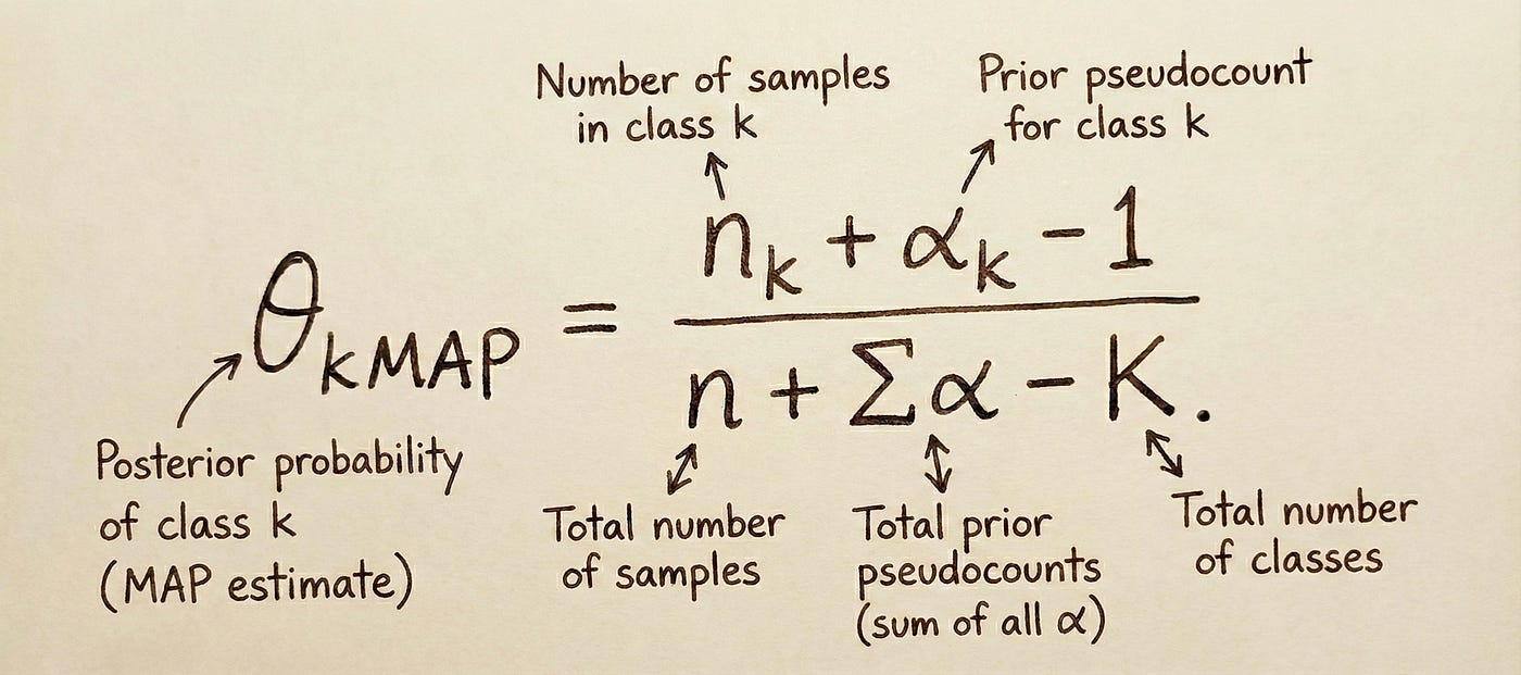
Let’s apply this to our previous example to see how adding the pseudo count alpha = 2 for each class (Additive Smoothing) avoids the zero-count and undefined probabilities.

This works pretty well on our previous example! but the issue is that our example is over simplified with only two features and two classes.

The hidden weakness of the Dirichlet-multinomial model is that it estimates a probability for every combination of features, which can result in making the model exponentially grow if we add more features and classes. This makes our model infeasible to store or train the data.

the Dirichlet-multinomial model complexity

This is called the curse of dimensionality, our attempt to model the full joint distribution of the data is too complex for many real world problems.

Naive Bayes’ Assumption with MAP Estimation

To fight the curse of dimensionality, we need a different strategy. Instead of modelling the full p(x|y), we can make a very simple assumption.

The Naive Bayes assumption states that All features are conditionally independent given the class y.

Naive Bayes Formula

So basically instead of one big probability table for all feature combinations like the Dirichlet multinomial model, we now have D number of small tables, one for each feature.

This is “Naive” because features are rarely truly independent in real world. However, the approach works pretty well in practice.

The number of parameters is now O(C D K), which is linear in the number of features D, not exponential. This makes the model simpler to store and train the data. The following shows the calculation steps of the Naive Bayes approach with MAP smoothing.

Bayesian Naive Bayes Approach

In the Bayesian naive bayes approach we still separate the features into individual tables, assuming linear independence but the smoothing is done using the Dirichlet multinomial posterior means which can be represented in the following formula:

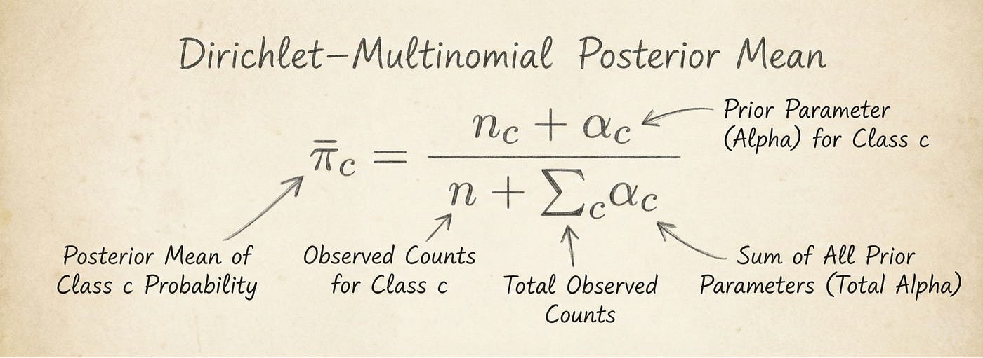
The following shows the calculation steps of the Bayesian Naive Bayes approach with posterior means smoothing.

Building on the previous results, we now calculate the conditional probability P(Rich | Young, CEO). While this calculation results to undefined using standard Maximum Likelihood Estimation (MLE), applying one of the three smoothing techniques allows us to find a valid, non-zero probability estimate.

References

• Swoboda, P. (2025/2026). Machine Learning [Lecture notes]. Department of Artificial Intelligence and Data Science, Heinrich Heine University Düsseldorf.
• K.P. Murphy. Probabilistic Machine Learning: An Introduction
• T. Mitchell. Machine Learning McGraw-Hill Education Ltd, 1997
• C.M. Bishop. Pattern Recognition and Machine Learning Springer, 2006
• I. Goodfellow, Y. Bengio, A. Courville. Deep Learning The MIT Press, 2017