If the Monty Hall Problem Had 1,000,000,000 Doors, How Would You Compute It?

I previously wrote about “What if the Monty Hall problem had two winning doors?” This time, I would like to formalize the problem so that we can handle arbitrarily large numbers of doors.

Once we have a formula, we can compute the outcome even if the number of doors is enormous.

Recap: The Classic Monty Hall Problem

• There are 3 doors and 1 prize.
• The player first chooses 1 door. The chance that this door is the winning door is 1/3.
• Among the remaining 2 doors:
• Either both are losing doors, or
• One is losing and the other is winning. In any case, there is at least one losing door among them.
• The host, who knows where the prize is, opens one losing door and reveals it.

Now the question is:

Is the remaining unopened door more likely to be the winning one than the player’s original door?

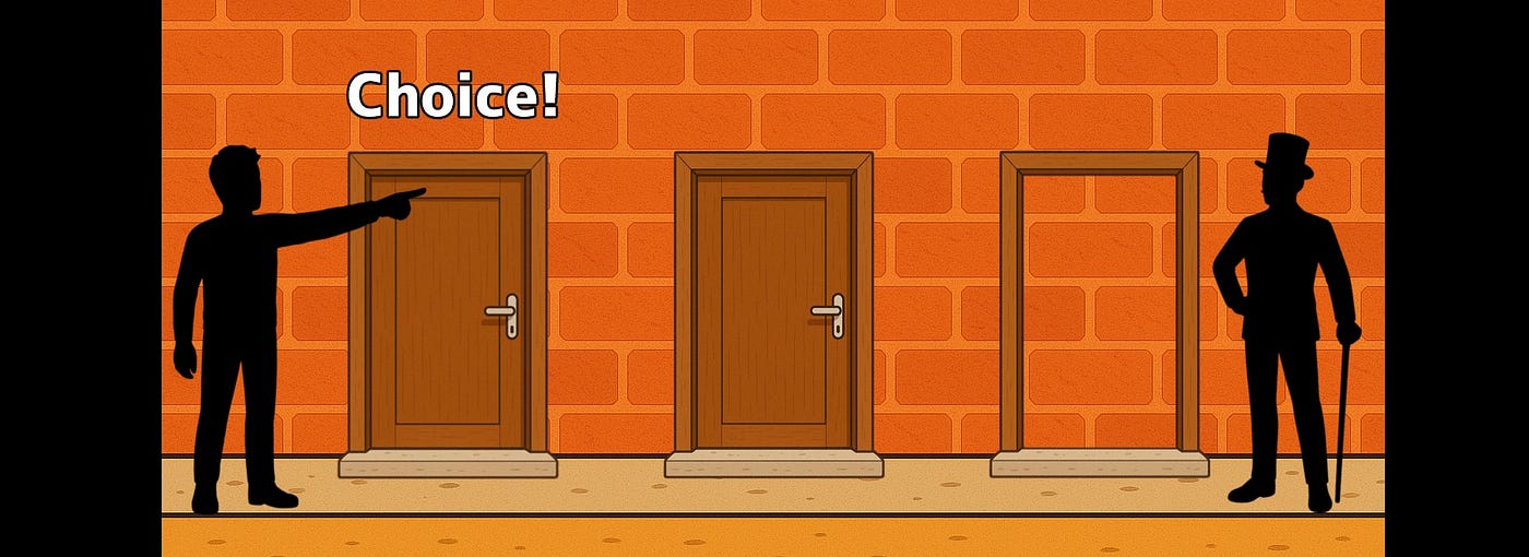
It’s better to change it!

The Aggregation Method

I am not very familiar with the literature, but I am sure many different formalizations of Monty Hall have been proposed.

Here, I would like to compute the probability of the remaining door using a method I will (somewhat arbitrarily) call the aggregation method.

First, treat each set of doors as a group.

On the first move, the doors are divided into two groups:

• Group p: the door initially chosen by the player The probability mass this group carries is:

number of winning doors​ / total number of doors

In the classic setting, this is 1/3.

The remaining doors are then split into two further groups:

• Group m: doors that the host will eliminate
• Group s: doors that remain as possible options for the player (the “switch” group)

The total probability mass carried by these two groups together is:

1 − p

In our classic setting, that is 1 − 1/3 = 2/3.

Divide the doors into three groups: p, m, and s

By construction of the game, group m always has probability 0 (the host always eliminates losing doors).

m is the probability of winning 0

Therefore, the entire 2/3 probability mass must belong to group s.

So the answer in the classic case is:

Switching group s: 2/3

The probability of s and m combined is 2/3. And if m=0%, then the answer is…

A 10-Door Variant

Now let us change the setup a bit.

• There are 10 doors.
• There are 2 winning doors.
• The player initially selects 2 doors.
• The host then eliminates 4 losing doors.
• At that point, 4 doors remain.

The player may either:

• Keep the originally chosen 2 doors, or
• Switch and select 1 of the 4 remaining doors.

The question is:

To maximize expected wins, should the player switch?

It’s a little much but it’s ok

This variant differs from the original in a few important ways:

1.We care about expected value, not just probability. In the classic problem, there is exactly one winning door, so “probability of winning” and “expected number of wins” coincide numerically. But when there are multiple winning doors, what matters is:

How many wins are expected in the chosen set?

This is the expected number of winning doors, not just a binary win/lose outcome.

We define the variables:

• n=10: total number of doors
• w=2: number of winning doors
• p=2: number of doors initially chosen by the player
• m=4 number of doors eliminated by the host
• s=1: number of doors the player may choose after switching

You can choose two doors at first, but after changing you can only choose one.

First, the expected number of wins per door is:

w/n = 2/10

The player initially chooses p=2 doors, so the initial expected number of wins in group p is:

2/10 + 2/10 = 4/10

So:

• Group p (initial choice) has expected wins: 4/10​.

Next, the host eliminates m=4 doors. By the rules of the game, all of these are guaranteed to be losing doors, so:

• Group m (doors eliminated by the host) has expected wins: 0.

That means the remaining expected wins:

w — 4/10 = 2 — 4/10 = 16/10

must be distributed among the remaining doors.

The number of remaining doors is:

n-p-m = 10–2–4 = 4

So the expected wins per remaining door is:

(2–4/10) / 10–2–4 = (16/10) / 4 = 4/10

So each of the 4 remaining doors carries expected wins of 4/10.

After switching, the player can choose only one of these remaining doors, so:

• Expected wins after switching: 4/10
• Expected wins staying with the original 2 doors: 4/10

Thus, switching and not switching are equivalent in terms of expected value in this particular setup.

The expected values ​​for groups p and s were the same

Deriving a General Formula

Let us generalize the above.

Let:

• n: total number of doors
• w: number of winning doors
• p: number of doors initially chosen by the player
• m: number of doors eliminated by the host
• s: number of doors the player may choose after switching

We will compute:

• E: expected number of wins after switching.

First compute the expected total number of wins in the doors the player did not initially choose:

• Total expected wins over all doors: w
• Expected wins in the initially chosen group p: w/n × p
• So expected wins in the remaining n − p doors:

w/n × (n — p)

Among those n − p doors, the host eliminates m doors, all of which are guaranteed to be losing doors, so the expected wins remain the same but are now concentrated into the remaining (n−p−m) doors.

So the expected wins per remaining door are:

The player then chooses s doors from this remaining set, so the expected number of wins after switching is:

In compact form:

The “Conservation of Expectation”

Conceptually, this method relies on what we might call the conservation of expectation (more precisely, the linearity of expectation).

We exploit two facts:

1. The host always eliminates doors with expected value 0 (guaranteed losers).
2. Therefore, the total expected number of wins remains the same, but is redistributed among fewer doors.

By grouping doors with similar roles and tracking how expectation moves between these groups, we can see how the “probability mass” shifts as the host acts.

If you have previously understood the Monty Hall problem intuitively, it was probably not via Bayes’ theorem, but through reasoning like:

“The probability the prize is in my original choice is fixed; the host’s reveal concentrates the remaining probability into the other group.”

The above formula is essentially a formalization of that intuitive “probability mass redistribution” idea.

The main cognitive stumbling block in Monty Hall is how to handle the host’s knowledge and intentional choice.

• If the host did not know where the prize is and eliminated doors at random, we could simply split probabilities uniformly.
• But since the host does know and intentionally avoids the prize, the usual “just divide evenly” approach breaks down.

Here, we handled that intentionality by:

• Treating “doors eliminated by the host” (group m) as having expected value 0, and
• Removing those doors from the pool over which expectation is distributed.

“Expectation Concentration”

In more intuitive language, when the host removes doors with expected value 0, the remaining doors experience a kind of:

Concentration of expectation

The total expected wins are the same, but they are packed into fewer doors.

Once we have the formula:

we can answer questions like:

“How many doors do I need to switch to so that switching becomes better than staying?”

just by plugging in the parameters.

Designing New Problems

We can also design more psychologically interesting variants. For example:

“If you win after switching, your prize is reduced by some factor.”

Then we can compare:

• The mathematically optimal strategy, and
• The strategy that “feels” right to most people,

and see how cognitive bias and expected value diverge.

The 1,000,000,000-Door Version

Finally, let us address the title case:

What if there are 1,000,000,000 doors?

First, we’ll have 1,000,000,000 doors.

Suppose:

• Total doors: n = 1,000,000,000
• Winning doors: w = 1,000,000
• Initial pick: p = 1,000,000 doors
• Host eliminates: m = 100,000,000 doors (all losing)
• After that, the player may switch and choose s = 100,000 doors.

First, compute the expected wins per remaining door after the host’s elimination:

Then multiply by the number of doors chosen after switching (s=100,000):

Eswitch ≈ 0.001111234705 × 100,000 ≈ 111.123

Now compare this with the expected wins in the initial 1,000,000 doors:

So:

In this setup, not switching yields a higher expected number of wins.

Since the expected wins per remaining door are approximately 0.001111234705, we can ask:

For which value of s does switching break even with staying?

Solve:

0.001111234705 × s = 1000 ⇒ s ≈ 899,899.9

So as long as the number of doors after switching s is 899,899 or fewer, staying is better. If s exceeds that threshold, switching becomes better in expectation.

Bonus: When Is Switching Better?

Let us derive the general condition for “switching is better than staying.”

We compare:

Expected wins after switching:

Expected wins if we stay:

We ask when:

Eswitch > Estay

Cancel w/n (assuming w>0):

Rewriting:

Whenever this inequality holds, switching yields a higher expected number of wins.

Caveats About the Formula

A few important notes about this formalization:

1. We are dealing with expected value, not simple probability. When there is exactly one winning door, expected wins and winning probability coincide numerically. When there are multiple winning doors, be careful:

• The formula gives expected number of wins, not the probability of “at least one win.”

2. The host must never eliminate a winning door. Formally, we require:

w ≤ n − p − m

That is, even in the worst case (the player’s initial picks are all losing), there must still be enough losing doors left for the host to eliminate m doors without touching any winning door.

This guarantees that the host’s eliminated group m has expected value 0, which is a key assumption in the derivation.

If that condition fails, then the host might be forced to eliminate winning doors, and the above formula would no longer apply.