IncSAR: Teaching SAR Models New Targets Without Forgetting the Old Ones

Most image recogition systems are trained once and then quietly deployed.

SAR target recognition does not get that luxury.

Military vehicles change. Sensor conditions shift. New target categories appear over time. Every new target category creates the same problem: how do you teach the model something new without wiping out what it learned last month?

That becomes much harder once you look at real SAR data instead of clean benchmark images.

SAR images do not behave like photographs. They are grainy, structurally sparse, and dominated by speckle patterns. In practice, two different vehicles can generate radar signatures that look almost identical, while the same vehicle can change appearance dramatically depending on viewing angle or acquisition conditions. Even building a standard classifier for SAR is already a nontrivial engineering problem.

Then continual learning enters the picture.

As new tasks arrive sequentially, the network starts drifting toward recently seen classes and older representations begin to collapse. Most continual learning systems handle this with replay buffers: keep samples from old tasks, mix them into future batches, and hope the feature space stays stable.

That assumption does not always hold in SAR pipelines, where storage budgets, deployment constraints, or dataset restrictions can make long-term image replay impractical.

IncSAR is built around exactly that constraint: incremental SAR recognition without relying on stored exemplars.

What makes the framework interesting is that it avoids the usual instinct to keep everything fully trainable.

Most of the heavy components stop learning surprisingly early in the process.

After the base phase, the focus shifts from retraining backbones to maintaining a stable representation space where new class statistics can be inserted incrementally.

Takeaway: IncSAR treats continual learning as a feature stability problem, not just a classification problem.

The Problem: Why SAR Incremental Learning Is Hard

Before looking at the architecture, it helps to clarify the exact continual learning setup the paper uses.

The paper uses class incremental learning (CIL).

Training begins with a base session containing a subset of target classes. After that, new classes arrive sequentially in tasks.

The catch:

• Old training images are no longer available
• The classifier must still recognize all previously seen classes
• Evaluation happens over the entire accumulated label space

So after Task 4, the model is tested on everything from Tasks 1 through 4 simultaneously.

This setup is already difficult in natural image datasets like CIFAR or ImageNet.

SAR makes it worse.

The paper highlights three major reasons:

• Smaller inter-class distances — different targets often produce visually similar radar signatures
• Larger intra-class distances — the same target can vary heavily across depression angles and acquisition conditions
• Speckle noise — SAR images contain multiplicative noise that corrupts fine texture details

In optical imagery, a pretrained backbone can often separate classes cleanly with little adaptation.

SAR does not behave that way.

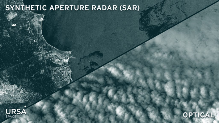
Figure 1 — Optical imagery versus SAR imagery.

The replay-buffer strategy used in many continual learning systems also becomes problematic here.

Replay introduces several issues:

• Old classes dominate memory over time
• Buffer balancing becomes difficult
• Storage grows continuously
• Some SAR datasets cannot legally or practically be retained

IncSAR makes a deliberate decision:

No rehearsal buffer.

Instead of storing images, it stores only compact prototype statistics.

That design choice ends up shaping the entire architecture.

Takeaway: IncSAR avoids replay entirely and replaces image memory with lightweight prototype statistics.

Figure 2 — The dual-branch design of IncSAR. The ViT branch provides stable global representations, while the SAR-CNN branch learns SAR-specific local structure. Incremental updates happen through prototype accumulation rather than image replay.

The Training Loop: Three Modes in One Codebase

One of the first interesting things in the repository is that IncSAR is not a single model.

The training loop supports three different variants controlled entirely through configuration flags.

The branching logic is surprisingly clean:

# trainer.py — the entry point decides which training mode to run
def train(args):
    for seed in seed_list:
        if args["late_fusion"] == True:
            acc_task, avg_acc = _train_late_fusion(args)    # IncSAR: dual branch, soft voting
        elif args["attention_fusion"] == True:
            acc_task, avg_acc = _train_attention_fusion(args) # IncSARLAtt: learned fusion
        else:
            acc_task, avg_acc = _train(args)                 # single branch baseline

The default IncSAR setup uses late_fusion=True.

This is where reading the actual training code becomes more useful than reading the abstract.

Inside _train_late_fusion(), the code never constructs a single unified hybrid model.

It builds two entirely independent pipelines.

# Two independent branches, each with its own hyperparameters
args_vit["backbone_type"] = args["backbone_type_vit"]
args_vit["rpca"]          = args["rpca_vit"]       # RPCA applied to ViT branch? (False)
args_vit["use_RP"]        = args["use_RP_vit"]     # random projection
args_vit["M"]             = args["M_vit"]          # projection dimension = 10,000

args_cnn["backbone_type"] = args["backbone_type_cnn"]
args_cnn["rpca"]          = args["rpca_cnn"]       # RPCA applied to CNN branch (True)
args_cnn["M"]             = args["M_cnn"]          # projection dimension = 10,000

The ViT branch and the SAR-CNN branch each get:

• Their own backbone
• Their own preprocessing
• Their own RPCA settings
• Their own DataManager
• Their own training loop

The branches are isolated almost all the way until inference.

Then the task loop runs both pipelines independently:

# For each incremental task, both models train independently
model_vit.incremental_train(data_manager_vit)
logits_vit, y_pred_vit, y_true = model_vit.eval_task_late_fusion()
model_vit.after_task()

model_cnn.incremental_train(data_manager_cnn)
logits_cnn, _, _ = model_cnn.eval_task_late_fusion()
model_cnn.after_task()

# Final prediction: softmax of each branch summed element-wise
cnn_accy = soft_voting(logits_vit, logits_cnn, y_true, args['init_cls'], args['increment'])

That final line is deceptively simple.

The system does not fuse intermediate feature maps.

It does not train a joint classifier.

It simply adds softmax outputs from both branches.

Which means the entire architectural philosophy is modular.

Each branch learns independently.

Fusion happens only at prediction time.

Takeaway: The dual-branch design is not just architectural — it’s structural. Two separate training pipelines, two separate DataManagers, fused only at prediction time.

SAR-CNN: Small on Purpose

The SAR-CNN branch is probably the most surprising part of the paper.

Instead of importing a massive pretrained CNN, the authors build a compact custom network trained directly on SAR data.

And the implementation is intentionally simple.

class custom_cnn(nn.Module):
    def __init__(self, in_features=3, out_features=10):
        super().__init__()
        self.conv16  = nn.Conv2d(3,   16,  kernel_size=7)  # large kernel to capture coarse SAR patterns
        self.conv32  = nn.Conv2d(16,  32,  kernel_size=5)
        self.conv64  = nn.Conv2d(32,  64,  kernel_size=5)  # note: 5×5 not 3×3
        self.conv128 = nn.Conv2d(64,  128, kernel_size=3)
        self.pool    = nn.MaxPool2d(kernel_size=2, stride=2)
        self.dropout = nn.Dropout(p=0.4)                   # heavy dropout — SAR data is limited
        self.flatten = nn.Flatten()

    def forward(self, x):
        x = F.relu(self.conv16(x));  x = self.pool(x)
        x = F.relu(self.conv32(x));  x = self.pool(x)
        x = F.relu(self.conv64(x));  x = self.pool(x)
        x = F.relu(self.conv128(x)); x = self.dropout(x)
        return self.flatten(x)  # output: 1152-dimensional vector for 70×70 input

A few details stand out immediately.

First, the kernels are larger than what you would expect in a modern CNN.

The network uses:

• 7×7
• 5×5
• 5×5
• 3×3

That is unusual in an era dominated by stacks of 3×3 convolutions.

But SAR images contain coarse scattering patterns rather than dense semantic textures. Larger receptive fields early in the network make sense.

There is also an interesting mismatch between the paper and the code.

The paper describes the third convolution layer as 3×3.

The actual implementation uses 5×5.

And when reproducing results, the implementation is what matters.

The parameter count is tiny by modern standards:

• Around 140K parameters total

Yet inside the IncSAR framework, this small network outperforms several massive backbones in ablation studies:

• DenseNet-121 (~7M params)
• ResNet-101 (~44M params)
• VGG-19 (~140M params)
• CLIP-ViT-L/14 (~303M params)

That result says something important about domain specialization.

Large pretrained vision models do not automatically transfer well when the underlying signal physics differs this much from natural imagery.

Takeaway: For a highly specialized domain like SAR, a small purpose-built CNN can outperform massive general-purpose models.

RPCA: Cleaning the Noise Before Learning

SAR images are noisy in a very specific way.

The speckle patterns are not simple Gaussian noise you can blur away with preprocessing.

They are multiplicative artifacts generated by coherent radar scattering.

That noise directly affects feature extraction.

IncSAR handles this using a learnable RPCA-style module integrated directly into the CNN branch.

The implementation is compact:

class BEAR_ABY(nn.Module):
    # Implements L = A B Y — a bilinear approximation of Robust PCA
    def __init__(self, inp, k=1):
        super().__init__()
        self.ln1 = nn.Linear(inp, k, bias=False)   # A: projects input to low-rank space (rank k)
        self.ln2 = nn.Linear(k, inp, bias=False)   # B: reconstructs back to original space

    def forward(self, x):
        L = self.ln2(self.ln1(x))   # L = low-rank component (background / noise)
        return L                     # caller computes X' = L - X (the sparse/clean component)

    def clamper(self):
        for p in self.parameters():
            p.data.clamp_(0.0)      # enforces non-negativity

Despite the RPCA terminology, the underlying mechanism is fairly straightforward once you follow the tensor flow.

First, the SAR image is reshaped into a vector representation.

Then:

1. ln1 projects the input into a very small low-rank subspace
2. ln2 reconstructs the smooth background component
3. The residual X' = L - X isolates the sparse target structure

So instead of learning directly from the raw SAR image, the CNN sees the residual emphasizing target information.

Another subtle design choice matters here.

The RPCA module is trained only during the base task.

After that, it freezes permanently.

No future adaptation.

No continual retraining.

The module becomes a fixed SAR filter shared across all future tasks.

That matters because the entire continual learning pipeline depends on feature consistency.

If preprocessing changed every task, prototype statistics would drift.

Freezing RPCA stabilizes the representation space.

Takeaway: RPCA isn’t a preprocessing step bolted on — it’s trained jointly with the CNN during the base task and becomes a fixed filter for all future tasks.

SSF: Adapting a Frozen ViT to SAR

The ViT branch faces a completely different problem.

The transformer backbone starts from ViT-B/16 pretrained on ImageNet.

Those pretraining statistics come from everyday RGB imagery — objects, animals, textures, and scenes that look nothing like radar returns.

It contains zero SAR images.

So the model starts with a major distribution mismatch.

IncSAR solves this with SSF — Scale Shift Fine-tuning.

The implementation is minimal:

def init_ssf_scale_shift(dim):
    scale = nn.Parameter(torch.ones(dim))    # initialized to 1 (identity)
    shift = nn.Parameter(torch.zeros(dim))   # initialized to 0 (identity)
    nn.init.normal_(scale, mean=1, std=.02)
    nn.init.normal_(shift, std=.02)
    return scale, shift

def ssf_ada(x, scale, shift):
    # Applies element-wise: x_out = x * scale + shift
    return x * scale + shift

Instead of updating the full transformer, the method learns only two vectors:

• Scale
• Shift

One value per feature dimension.

The clever part is where SSF gets inserted.

def forward(self, x):
    # SSF modulates the input AFTER LayerNorm, BEFORE Attention
    x = x + self.drop_path1(
        self.ls1(self.attn(ssf_ada(self.norm1(x), self.ssf_scale_1, self.ssf_shift_1)))
    )
    # SSF also applied before MLP
    x = x + self.drop_path2(
        self.ls2(self.mlp(ssf_ada(self.norm2(x), self.ssf_scale_2, self.ssf_shift_2)))
    )
    return x

SSF operates:

• After LayerNorm
• Before Attention
• Before the MLP block

The pretrained ViT weights themselves stay frozen.

Only these lightweight modulation parameters adapt to SAR.

That dramatically reduces the number of trainable parameters while preserving ImageNet-learned global representations.

The ablation results are large enough to matter:

• Frozen ViT without SSF: 76.87% last-task accuracy
• Adding SSF + random projection + LDA improves performance by 27%

Which suggests the pretrained features were useful — but badly calibrated for SAR until SSF corrected them.

Takeaway: SSF turns a frozen ImageNet model into a SAR-aware feature extractor by learning just two numbers per feature dimension — scale and shift.

Attention Fusion: The IncSARLAtt Variant

The standard IncSAR system uses soft-voting late fusion.

Simple.

Fast.

Modular.

But the repository also contains a more sophisticated variant called IncSARLAtt.

Instead of combining class probabilities, it learns feature fusion directly using attention.

The implementation looks like this:

class attention_layer(nn.Module):
    def __init__(self, emb_dim=672, tf_layers=4, tf_head=8, tf_dim=336,
                 activation="gelu", dropout=0.1, pre_norm=True):
        super().__init__()
        self.emb_dim = emb_dim
        self.cls_token = nn.Parameter(torch.randn(self.emb_dim))  # learnable CLS token

        self.transformer = nn.TransformerEncoder(
            nn.TransformerEncoderLayer(
                d_model=emb_dim,         # 672 — chosen to fit concatenated ViT-Ti + SAR-CNN features
                nhead=tf_head,           # 8 attention heads
                dim_feedforward=tf_dim,  # 336 (half of emb_dim)
                batch_first=True,
                norm_first=pre_norm,     # Pre-LN for training stability
            ),
            num_layers=tf_layers,        # 4 layers
        )

    def forward(self, x_vit, x_cnn):
        x = torch.cat([x_vit, x_cnn], dim=1)         # concatenate both branch features
        x = x.reshape(x.shape[0], -1, self.emb_dim)
        cls_token = self.cls_token.expand(x.shape[0], 1, -1)
        x = torch.cat((cls_token, x), dim=1)          # prepend CLS token
        x = self.transformer(x)
        return x[:, 0, :]                              # use only CLS token output for classification

The CLS-token design mirrors BERT and ViT itself.

The transformer learns how to aggregate information from:

• The ViT branch
• The SAR-CNN branch

into one shared representation.

This becomes especially important during cross-domain experiments.

When the tasks shift dramatically across aircraft, vehicles, and ships, the relative usefulness of each branch changes.

The attention mechanism can adaptively reweight them.

And the results support that interpretation.

Cross-domain forgetting drops to just 3.08%, compared to 5.42% for standard IncSAR.

So while late fusion is cheaper, attention fusion appears more robust under strong distribution shifts.

Takeaway: Attention fusion is more expensive but learns to dynamically weight features from both branches — which matters most when the target domain shifts across tasks.

Prototype Learning and Random Projection

The continual learning component of IncSAR is refreshingly different from replay-heavy methods.

Instead of storing images, the framework stores only prototype statistics.

The pipeline works like this:

1. Features are extracted using frozen backbones
2. Features are projected into a 10,000-dimensional space
3. Class statistics accumulate incrementally
4. Prototypes become the classifier

The random projection step is important.

A fixed random matrix W maps features into a high-dimensional space.

That matrix is initialized once.

Then frozen forever.

Nothing about it is learned.

After projection, the framework accumulates:

• Gram matrix G
• Prototype matrix C

Then computes decorrelated prototypes:

P = (G + λI)⁻¹ C

where λ is a ridge regularization parameter optimized using an 80/20 split of task data.

The key design constraint is stability.

Because:

• The CNN freezes after base training
• RPCA freezes after base training
• The ViT backbone freezes
• The projection matrix freezes

all future tasks exist in a consistent feature space.

That consistency is what makes exemplar-free learning possible.

The framework never needs to revisit old images because the representation geometry itself stays stable.

That is a very different philosophy from methods that continually fine-tune the backbone.

Takeaway: Random projection into 10K dimensions + frozen backbone = a consistent feature space where prototype statistics can be updated incrementally without any stored images.

Results That Matter

The results are interesting not just because the accuracies are high, but because forgetting stays extremely low without exemplars.

MSTAR B4Inc1

This setup starts with 4 base classes and introduces 1 class per incremental task.

Results:

• IncSAR: 99.27% average accuracy, 0.78% performance drop
• IncSARLAtt: 99.34% average accuracy
• Compared to FOSTER, IncSAR reduces performance drop by 81%

MSTAR B2Inc2

This version introduces 2 classes per task.

Results:

• IncSARLite: 99.7% average accuracy
• Performance drop: just 0.62%

An important detail here is that competing systems like HPecIL and MLAKDN rely on stored exemplars.

IncSAR does not.

Cross-domain experiments

The hardest experiments involve sequential domain shifts:

• Aircraft
• Vehicles
• Ships

Results:

• IncSAR: 96.78% average accuracy
• IncSARLAtt achieves the lowest forgetting with a 3.08% drop

Compute comparison

The lightweight variants are arguably the most interesting part.

• IncSAR: 106M parameters, 17.62G MACs
• IncSARLite: 21M parameters, 22.9% faster training
• IncSARLAtt: 17M parameters, 74% faster training than IncSAR

And despite being smaller, the lightweight variants sometimes outperform the heavier baseline.

That is usually a sign the architecture is better aligned with the task distribution.

Takeaway: The lightweight variants don’t just reduce compute — in several setups, they actually outperform the heavier base model.

What This Actually Means

The most important idea in this paper is not the benchmark score.

It is the architectural philosophy.

A lot of modern transfer learning assumes that a giant pretrained transformer can eventually adapt to almost any domain.

IncSAR takes a more careful position.

The authors treat the ImageNet-to-SAR gap as fundamentally real.

Instead of trying to force a ViT to fully become a SAR model, the framework splits responsibilities.

The ViT branch handles:

• Global semantic structure
• Long-range relationships
• General representation power

The SAR-CNN branch handles:

• Speckle-aware local structure
• Domain-specific radar patterns
• Noise-sensitive texture extraction

The branches complement each other instead of competing.

And then comes the more subtle design decision.

After the base task, nearly everything freezes.

The backbones stop updating.

RPCA stops updating.

The random projection matrix stops updating.

Incremental learning becomes mostly about maintaining stable prototype statistics.

That is why the system can remain exemplar-free while still controlling forgetting.

And honestly, that may be the broader lesson beyond SAR.

Sometimes the right way to solve a difficult continual adaptation problem is not to keep training bigger and bigger networks forever.

Sometimes the better strategy is:

• Freeze the expensive representation layers early
• Build a stable feature space
• Let a lightweight memory mechanism handle incremental updates

That design philosophy is what makes IncSAR worth studying.

Reference Links

• GitHub: https://github.com/geokarant/IncSAR-A-dual-fusion-incremental-learning-framework-for-SAR-Target-Recognition
• Paper: https://ieeexplore.ieee.org/document/10838563