🚀 Amazon Redshift Node Types Explained: RA3, DC2, DS2, and DC1 Made Surprisingly Simple

How Amazon Redshift evolved from fixed storage to intelligent managed storage — and why choosing the right node can save both money and headaches.

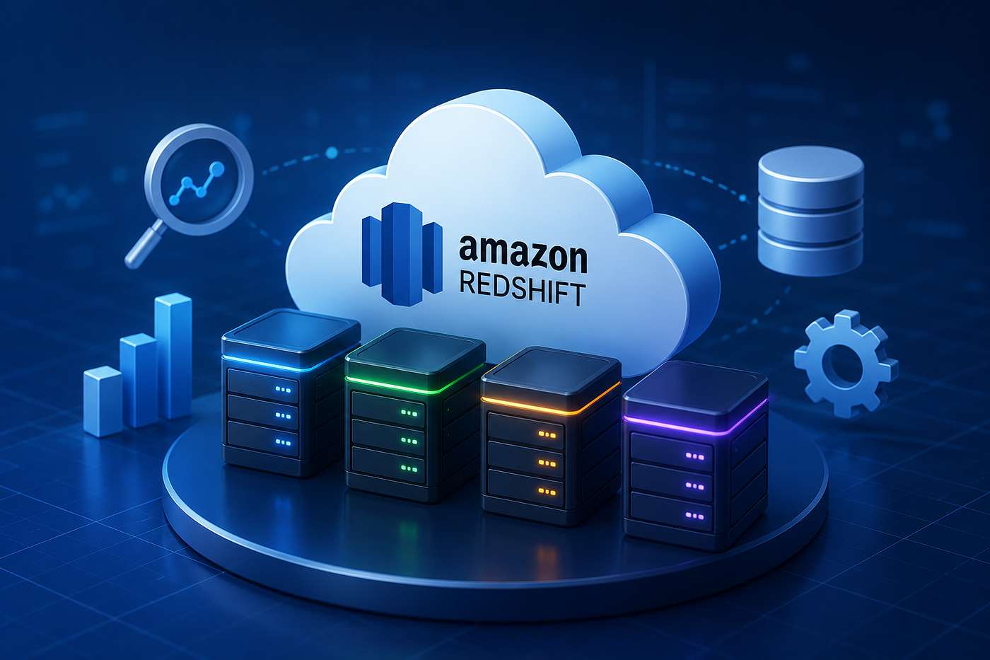
Imagine you’ve just created your first Amazon Redshift cluster.

AWS asks you to choose a node type:

• RA3
• DC2
• (Maybe you’ve even heard about DS2 or DC1)

If you’re new to Amazon Redshift, these names don’t explain much. They sound more like robot models than cloud infrastructure.

Most beginners immediately start wondering:

“What exactly is a Redshift node?”

“Why are there multiple node types?”

“What is Managed Storage?”

“Why does everyone recommend RA3 today?”

These are excellent questions because choosing the wrong node type can affect your warehouse’s performance, scalability, and even your AWS bill.

So instead of memorizing feature tables, let’s understand the story behind these node types.

By the end of this article, you’ll know not only what each node does but why AWS designed them this way.

First Things First: What Exactly Is a Redshift Node?

Before comparing node types, let’s understand one simple idea. Think of an Amazon Redshift cluster as a company. Every company has different employees doing different jobs. A Redshift cluster works in a similar way.

There are two types of nodes:

• Leader Node
• Compute Nodes

The Leader Node acts like a project manager. It doesn’t actually analyze data itself.

Instead it:

• Receives your SQL query
• Breaks it into smaller tasks
• Assigns those tasks to compute nodes
• Collects the results
• Returns the final answer

The heavy lifting happens inside the Compute Nodes.

These nodes:

• Store your data
• Execute SQL queries
• Perform joins
• Run aggregations
• Process millions (or even billions) of rows in parallel

When AWS talks about RA3, DC2, DS2, or DC1, it’s referring to these compute nodes — not the leader node.

Why Are There Different Node Types?

Imagine buying a laptop. Every laptop comes with:

• A processor (CPU)
• Memory (RAM)
• Storage (SSD)

Different people need different combinations.

• A video editor may want huge storage.
• A software developer may need more RAM.
• A student may simply want an affordable laptop.

Similarly, not every company using Redshift has the same requirements.

Some organizations have:

• Small datasets
• Massive petabytes of historical data
• Fast-growing warehouses
• Stable workloads that rarely change

Instead of forcing everyone to use one type of hardware, AWS introduced multiple generations of nodes over the years. Each generation solved problems that existed in the previous one.

Let’s travel through that evolution.

The First Generation: DC1 Nodes

When Amazon Redshift was first introduced, AWS launched DC1 (Dense Compute) nodes. These nodes focused on delivering fast query performance using local SSD storage. Everything a node needed was inside one machine:

• CPU
• RAM
• SSD Storage

This design worked well because SSDs were much faster than traditional hard drives. However, there was one major limitation. Suppose your warehouse had enough processing power but eventually ran out of storage. Could you simply buy more storage? Unfortunately, no. You had to purchase an entirely new node. That meant paying for additional CPUs and memory even if you didn’t need them. It was similar to buying an entirely new laptop just because your existing laptop’s SSD became full. While DC1 was a great starting point, AWS knew there was room for improvement.

The Storage-Focused Generation: DS2 Nodes

Not every business prioritizes speed. Some organizations simply need to store enormous amounts of data as economically as possible. To solve this problem, AWS introduced DS2 (Dense Storage) nodes. Instead of SSDs, DS2 nodes used traditional hard disk drives (HDDs). Hard drives are slower than SSDs but offer significantly more storage for the same cost. This made DS2 ideal for organizations that stored huge historical datasets and didn’t require lightning-fast query performance.

You can think of DS2 as a warehouse. It can hold a tremendous amount of inventory, but retrieving that inventory takes longer than opening a drawer in your office. For businesses with archival or infrequently accessed data, DS2 offered a practical balance between capacity and cost.

A Better Compute Generation: DC2 Nodes

Technology never stands still. AWS later introduced DC2 (Dense Compute) nodes as the successor to DC1. Like DC1, DC2 continued using local SSD storage, but with newer hardware, faster processors, and improved performance. For many years, DC2 became the preferred choice for analytics workloads where datasets comfortably fit on local SSDs.

However, one important limitation still remained. Storage and compute were permanently tied together. Imagine your warehouse currently looks like this:

• 8 CPU cores
• 32 GB RAM
• 2 TB SSD

Now your business grows. Your data increases from 2 TB to 6 TB. Did your queries suddenly require more CPU? Probably not. You simply needed more storage. But with DC2, you couldn’t expand storage independently.

Your only option was adding more nodes, which automatically increased:

• CPU
• Memory
• Storage

Even when you only needed storage. This worked — but it wasn’t always cost-effective. AWS realized there had to be a smarter approach.

Enter RA3: The Biggest Evolution in Amazon Redshift

RA3 wasn’t just another hardware upgrade. It completely changed how Redshift stores data. Instead of tightly coupling storage with compute, AWS separated them. This idea is called decoupling compute and storage, and it’s one of the biggest architectural improvements in Redshift’s history.

Here’s what an RA3 node contains:

• CPU
• Memory
• High-speed SSD cache

But here’s the interesting part. It doesn’t try to store all of your data locally. Instead, most of your data lives in something called Amazon Redshift Managed Storage.

So, What Is Redshift Managed Storage?

Managed Storage is exactly what its name suggests. AWS manages your warehouse storage for you. Instead of requiring you to decide which files belong on SSDs or slower storage, Redshift continuously monitors how your data is being used.

Frequently accessed tables are automatically kept on high-performance local SSDs. Older or less frequently used data is automatically stored in Amazon S3-backed managed storage. You don’t move data manually. You don’t configure storage tiers. You don’t even notice it happening.

Redshift intelligently handles everything behind the scenes. Imagine a library. The books students borrow every day stay on shelves near the entrance. Books that are rarely requested are moved into a storage room. When someone eventually asks for an old book, the librarian retrieves it and places it back near the front if it starts becoming popular again.

That’s essentially how Managed Storage works.

Why Is RA3 Such a Big Deal?

Let’s imagine a company stores 100 TB of sales data. Employees regularly query only the most recent 5 TB. With older node types, all 100 TB had to occupy expensive local storage. With RA3, only the frequently accessed data remains cached locally, while the remaining data stays in managed storage.

The result? Lower costs. Better flexibility. And easier scaling. Need more storage? Simply pay for additional managed storage. Need more processing power? Scale compute independently. No wasted resources. No unnecessary hardware.

Which Node Type Should You Choose?

If you’re creating a new Redshift cluster today, the answer is surprisingly straightforward. For most modern workloads, RA3 is the recommended choice.

Its ability to separate storage from compute gives organizations far greater flexibility while keeping costs under control. DC2 still has its place.

If your dataset is relatively small, fits comfortably on local SSDs, and isn’t expected to grow significantly, DC2 can still provide excellent performance. DS2 and DC1, on the other hand, are largely part of Redshift’s history. They played an important role in Redshift’s evolution, but newer architectures have largely replaced them for new deployments.

A Simple Way to Remember Everything

Whenever you feel confused about node types, remember this analogy.

Imagine you’re buying computers for an office.

With DC2, every time employees need more storage, you buy entirely new computers — even though the existing computers are powerful enough.

With RA3, employees keep using the same computers, but you simply expand cloud storage whenever needed. Same processing power. More storage. Much lower waste.

That single idea explains why RA3 has become the preferred architecture for Amazon Redshift.

Final Thoughts

Amazon Redshift node types aren’t just different hardware options — they represent the evolution of cloud data warehousing itself.

AWS moved from tightly coupled infrastructure, where storage and compute always grew together, to a smarter architecture where each can scale independently.

Understanding this journey makes the node names much easier to remember:

• DC1 introduced fast SSD-based compute nodes.
• DS2 focused on affordable, high-capacity storage.
• DC2 improved performance while keeping compute and storage together.
• RA3 revolutionized Redshift by introducing Managed Storage, allowing compute and storage to scale independently.

The next time someone asks, “Why is everyone recommending RA3?” you’ll know the answer isn’t just because it’s newer.

It’s because it solves one of the biggest challenges in data warehousing: growing storage without forcing you to buy compute you don’t need.

Thousands of developers share what they’re building, learning, and discovering across our publications every month. One account connects you to our entire network of publications and communities. Explore more at plainenglish.io.