Decoding the Common Confusions

“Clarifying Deep Learning: Exploring Confusing Terms for Better Understanding”

As a beginner and self-learner in deep learning, each day introduces you to a bunch of new concepts to grasp. With each article that you click on, come a lot of new terms, and this is where confusions arise. It is very easy to misunderstand or not clearly see the difference between a few terms, that might be related.

Having faced these challenges myself, I am here, for the rescue. It’s time to demystify some common misconceptions (as a beginner) and gain a clearer understanding of key concepts in deep learning.

Table of Contents

1. Convolution v/s Matrix Multiplication
2. Global Average Pooling v/s Flattening
3. Activation Map v/s Feature Map v/s Attention Map
4. Epoch v/s Iteration v/s Batch
5. Data Augmentation v/s Regularization
6. Learning Rate v/s Momentum
7. Vanishing Gradient v/s Exploding Gradient
8. Encoding v/s Embedding
9. Bias v/s Variance
10. Early Stopping v/s Convergence

CONVOLUTION v/s MATRIX MULTIPLICATION

Both convolution and matrix multiplication are fundamental linear operations in the domain of neural networks, but both serve a different purpose. In the image provided below, the 1st matrix, i.e. [[1 2], [4 5]] would be treated as the input.

Convolution: You can visualize this better ***here***.

• Usage: Convolution is an essential operation in CNNs. Here, a small matrix called filter/kernel is made to slide over the input matrix/image, which in-turn detects patterns and extracts features.
• Output: The output of a convolution operation is generally smaller than the input. It is determined using the parameters like filter size, padding and stride values.
• Example: In image processing, convolution is used for tasks like edge detection, blurring, and feature extraction.

Matrix Multiplication: You can visualize this better here.

• Usage: Matrix multiplication is an extensively used operation in neural networks. It is used to calculate the dot product of weights and inputs, followed by applying activation functions.
• Output: The output of matrix multiplication depends on the dimensions of the matrices involved (following the rules of matrix algebra).
• Example: In a fully connected layer of a neural network, matrix multiplication is used to compute the weighted sum of inputs from the previous layer.

Source: created by me

GLOBAL AVERAGE POOL v/s FLATTEN

Both global average pooling and flatten are two different ways of reducing the dimensionality of a feature map, to prepare them for input into fully connected layers. Both are typically employed before fully connected layers in CNNs. Now, which method we should use depends on the specific needs of our model.

Global Average Pooling:

• Usage: Global average pooling computes the average value of each feature map across its spatial dimension (height and width). This operation results in a single value for a feature map, and ultimately in a 1d vector. Global average pooling helps in reducing the number of parameters in the network; providing a more compact representation of features, and also reducing overfitting. However, it may lose some spatial information.
• Output: The output of global average pooling is a vector with a fixed number of elements (same as the number of channels), where each element represents the average activation of a single feature map.

Source: GAP

Flatten Operation:

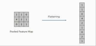
• Usage: The flatten operation is used to convert multidimensional feature maps (or arrays) into a 1d vector, to prepare it for the subsequent fully connected layers. Here, all the dimensions of the feature maps are concatenated into a single vector, effectively “flattening” the structure.
• Output: The output of the flatten operation is a 1d vector containing all the elements of the input array in a linear order.

Source: Flattening

ACTIVATION MAP v/s FEATURE MAP v/s ATTENTION MAP

The terms “feature map,” “activation map,” and “attention map” are often used in the context of neural networks, particularly in CNNs. Here’s more detail on each of them.

Feature Map:

• Definition: Feature maps are the outputs of a convolutional layer, generated by convolving the input data with learned filters/kernels, and each feature map represents the activation of a specific filter applied to the input data. Feature maps in CNNs represent various image features, such as edges, textures, and object parts, which may be crucial for subsequent layers to learn complex patterns and ultimately make accurate predictions.
• Usage: Feature maps capture hierarchical representations of input data, starting from low-level features (such as edges and textures) in initial/starting layers to high-level features (such as object parts or context or concept) in deeper layers.

Activation Map:

• Definition: An activation map, also known as a feature activation/response map, refers to the spatial distribution of activations within a feature map after applying an activation function. After convolutional layers in a CNN, activation functions (such as ReLU, tanh, sigmoid etc.) are applied element-wise to feature maps. These activations introduce non-linearities and enhance the model’s expressive power.
• Usage: Activation maps visualize how different parts of a feature map are activated or suppressed based on the learned patterns and weights of the neural network. In object detection tasks, activation maps can highlight regions of the input image where objects or features of interest are detected with high activation values, aiding in localization and segmentation tasks.

Attention Map:

• Definition: An attention map, often associated with attention mechanisms in deep learning, represents the importance or relevance of different parts of an input sequence or image. In machine translation tasks, attention maps visualize which words in the input sequence are given more attention to, when generating each word in the output sequence.
• Usage: Attention mechanisms allow the model to focus on relevant information while ignoring irrelevant or noisy parts of the inputs. Attention maps are commonly used in sequence-to-sequence models (NLP and image captioning tasks) to improve performance by selectively attending to important features (or tokens).

EPOCH v/s ITERATION v/s BATCH

Epoch:

• Definition: An epoch refers to one complete pass through the entire training dataset during the training phase of a model. During each epoch, the model sees and learns from all the training samples given in the dataset, and updating its parameters (weights and biases) based on the observed patterns and errors.
• If you train a neural network for 5 epochs on a dataset with 1000 samples, it means the model will iterate through the entire dataset 5 times, adjusting its parameters after each pass to minimize the training loss.

Iteration:

• Definition: An iteration, also known as a training step or batch iteration, refers to one update of the model’s parameters based on a batch of training examples. Iterations allow the model to learn from a subset of the training data at a time, making the training process computationally efficient and suitable for large datasets.
• During each iteration, the model computes predictions for a batch of input data, compares these predictions to the actual targets, calculates the loss, and updates the model’s parameters using an optimization algorithm.

Batch:

• Definition: A batch is a subset of the dataset processed in one go. The number of training samples in one iteration is referred to as the “batch size”.

In machine learning, an epoch is a complete pass through a dataset, while an iteration is the number of steps or batches needed to complete one epoch.

DATA AUGMENTATION v/s REGULARIZATION

Both data augmentation and regularization are the techniques that are used to improve a model’s performance. Both can reduce a model’s variance. Data augmentation is a way to expand a dataset, while regularization aim to prevent overfitting (by controlling the complexity of the model or adding constraints to the optimization process). Data augmentation is often presented as a type of regularization in deep learning. Let’s dive deeper.

Data Augmentation:

• Definition: It is a technique used to artificially increase the size of a training dataset, by applying various transformations (like crop, rotation, resize, mix-up, brightness, contrast, adding noise etc.) to existing data samples. It aims at is bringing diversity and variability into the training data and as a result, helps in improving the generalization ability of the models.
• Usage: Data augmentation is widely used in image classification, object detection, and other computer vision tasks, where having a diverse training dataset can lead to more robust and accurate models.

Source: Data augmentation

Regularization:

• Definition: It refers to a certain set of techniques used to prevent overfitting in ML/DL models, by imposing constraints or modifying the optimization process. It adds a penalty term to the model’s loss function to do so. Regularization mainly focuses on reducing the model’s complexity and encourage simpler solutions that generalize better to unseen data.
• Usage: Regularization is applied during the training phase to penalize complex model architectures, thereby discouraging the model from memorizing noise or learning irrelevant patterns in the training data.
• Common regularization techniques include L1 regularization (Lasso), L2 regularization (Ridge), dropout, dropconnect, early stopping, batch normalization, elastic-net regularization, data augmentation, adversarial training, weight decay and weight pruning etc.

LEARNING RATE v/s MOMENTUM

Learning rate and momentum are two important hyperparameters used in model optimization for training neural networks.

Learning Rate:

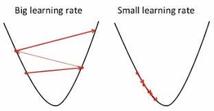
• Definition: The learning rate is a hyperparameter used during model optimization, that controls the size of steps that should be taken to update the model parameters (e.g., weights and biases), in the direction that reduces the loss function. It influences the convergence speed and stability of the model and the optimization process. A higher learning rate can lead to faster convergence but there are risk of it overshooting the optimal solution or oscillating around it. On the other hand, a lower learning rate may result in slower convergence, but is also capable of leading to stable and accurate updates.
• The learning rate is typically adjusted during training, using techniques like learning rate schedules (i.e. changing the learning rate over time) or adaptive learning rate algorithms (e.g., Adam, RMSProp etc.) that itself adjust the learning rate, based on the magnitude of the gradient and past information.

Source: Learning rate

Momentum:

• Definition: Momentum aims at improving convergence. It enhances the optimization process by introducing inertia or momentum to the gradient descent updates — meaning that the algorithm tends to keep moving in the direction where the gradients have been consistently pointing, which can help overcome local minima and speed up convergence. This allows the optimization algorithm to accumulate velocity in directions of consistent gradients. Momentum also helps dampen oscillations or noise in the parameter updates.
• A higher momentum value increases the influence of past gradients on the current update, leading to smoother and more stable optimization trajectories. However, too high a momentum value can also cause overshooting or instability in the optimization process. Common values for momentum range from 0.8 to 0.99, with 0.9 being a commonly used default value.

Source: Momentum

VANISHING GRADIENT v/s EXPLODING GRADIENT

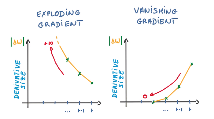
• Vanishing gradients occur when with subsequent updates, the gradients get smaller and smaller, gradually approaching zero. This can cause the weights of the initial layers to remain nearly unchanged, which can prevent the gradient descent from converging.
• Exploding gradients occur when the gradient continues to get larger. This can cause large weight updates, which can cause the gradient descent to diverge or keep oscillating between values and thus preventing it from converging.

Source: https://www.comet.com/site/blog/vanishing-exploding-gradients-in-deep-neural-networks/

ENCODING v/s EMBEDDING

Encoding:

• Definition: Encoding refers to the process of representing data (text, images, or numerical data) into a numerical format that can be easily manipulated, analyzed, or fed into machine learning algorithms for various tasks such as classification, regression, or generation.
• There are different types of encoding methods based on the type of data: Text Encoding (converting words or sentences into numerical representations), Image Encoding (converts image data into numerical arrays or feature vectors), Numerical Encoding (may involve normalization, scaling).

Embedding:

• Definition: Embedding refers to the process of learning a dense, lower-dimensional representation (embedding vector) of high-dimensional data, such as words, sentences, or images, using techniques like word embeddings or feature embeddings. Embeddings capture semantic relationships, contextual information, and similarities between data points in a continuous vector space, enabling models to generalize better and capture meaningful patterns.
• Example: Word embeddings like Word2Vec represent words as dense vectors in a continuous vector space, where similar words have similar vector representations.

BIAS v/s VARIANCE

• Bias refers to the error introduced by approximating a real-world problem with a simplified model or algorithm that does not capture the underlying complexity of the data. It measures how well a model captures the true relationships in the data — High bias tends to oversimplify the data and make strong assumptions or biases about the relationships between features and the target variable and hence can lead to underfitting.
• Variance refers to the sensitivity of a model’s predictions to changes in the training dataset, indicating how much the model’s performance varies across different training sets. It measures how much a model’s predictions vary across different training sets — High variance model is overly sensitive to fluctuations in the training data and tends to capture noise or random fluctuations as if they were meaningful patterns and hence can lead to overfitting.

Techniques like cross-validation, regularization, and model selection help address bias-variance trade-offs and improve model performance.

EARLY STOPPING v/s CONVERGENCE

Early Stopping:

• Definition: Early stopping is a regularization technique used during the model training, to prevent overfitting and improve generalization. It monitors the model’s performance on a validation dataset during training. If the validation loss does not decrease for several consecutive epochs, it indicates that further training may lead to overfitting and training is put to a halt.
• It involves monitoring a chosen metric (such as validation loss or accuracy) over successive epochs and is typically implemented using callbacks or monitoring techniques.
• Early stopping can help find an optimal balance between model complexity and generalization by preventing the model from memorizing noise or irrelevant patterns in the training data.

Convergence:

• Definition: Convergence refers to the state in which a model has reached a point where further iterations or epochs do not significantly improve its performance on the training or validation data. Convergence is typically indicated by stable or decreasing training and validation loss curves over successive epochs, along with stable or improving performance metrics (accuracy or F1 score).

I believe, we are good to move ahead in our journey and ace Deep Learning. Happy Learning y’all!!