Implementing a Character-Level Language Model (Activations, Gradients, BatchNorm)— Part 3A

In Part 2, we implemented a Neural Probabilistic Language Model. This model is a simple neural network composed of three layers: an input layer that converts the input into embeddings using a lookup table, a hidden layer with tanh non-linearity, and an output layer that translates the hidden layer’s output into probabilities.

We aim to shift our focus towards more complex MLPs, such as Recurrent Neural Networks (RNNs). It’s important to note that RNNs are not as easily optimizable with the first-order gradient techniques available to us. Understanding why they present optimization challenges requires a grasp of how activations and their gradients behave during training. In this post, we’ll look dig deeper into activations and their gradients.

Fixing the initial loss

Our implemented network is inappropriately initialized, resulting in a very high initial loss (~27). The reason for this high loss is that the network is confidently wrong, assigning high probabilities to the incorrect next character. We aim to reduce this loss, allowing the network more cycles for effective learning.

In the training of neural nets, it is almost always the case that you will have a rough idea of what loss you can expect at initialization. That depends on the loss function and the problem setup.

Let’s calculate the initial loss for our network. Assuming the default initialization, where the model knows nothing about internal relationships, it should ideally assign equal probabilities to all characters. With 27 characters, the probability assigned to each should be 1/27 (0.037). The log loss would be-torch.tensor(1/27).log()i.e 3.2958.

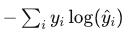
To calculate the loss for a single instance. y_i is true probability. y^_i is the predicted probability of ith class.

Our loss is high because our network, rather arbitrarily, assigns very high probabilities to the incorrect label (or low probability to the correct label).

# Assign high probability to incorrect label will cause higher loss.
logits = torch.tensor([5.0, 0.0, 0.0, 0.0, 0.0, 0.0, 0.0, 0.0, 0.0, 0.0, 0.0, 0.0, 0.0, 0.0, 0.0, 0.0, 0.0, 0.0, 0.0, 0.0, 0.0, 0.0, 0.0, 0.0, 0.0, 0.0, 0.0])
probs = torch.softmax(logits, dim=0)
loss = -1 * torch.log(probs[2])
probs, loss
"""(tensor(
[0.8509, 0.0057, 0.0057, 0.0057, 0.0057, 0.0057, 0.0057, 0.0057, 0.0057,
 0.0057, 0.0057, 0.0057, 0.0057, 0.0057, 0.0057, 0.0057, 0.0057, 0.0057,
 0.0057, 0.0057, 0.0057, 0.0057, 0.0057, 0.0057, 0.0057, 0.0057, 0.0057]),
tensor(5.1614))"""

For initialization, we want roughly equal values for all logits. This would assign equal probabilities to all output labels. We’ll start with zero values for the logits to avoid arbitrary high or low values.

We can make logits coming closer to the zero, by making W2 = 0 (roughly) & b2 = 0. This will results into logits that are closer to zero at initialization, thus avoiding being confidentaly wrong. Here is the updated code (only W2 and b2 initializations are changed)

# -------------------------- Initializations ------------------------
n_embd = 10                             # The dimensionality of the character embedding vectors
n_hidden = 200                          # The number of neurons in the hidden layers of the MLP
vocab_size = len(itos)

g = torch.Generator().manual_seed(2147483647)                         # for reproducibility
C = torch.randn((vocab_size, n_embd),                 generator=g)
W1 = torch.randn((n_embd*block_size, n_hidden),       generator=g)
b1 = torch.randn(n_hidden,                            generator=g)
W2 = torch.randn((n_hidden, vocab_size),              generator=g) * 0.1  # Scale down. Dont be confidentally wrong at initialization. 
b2 = torch.randn(vocab_size,                          generator=g) * 0

parameters = [C, W1, b1, W2, b2]
print(sum(p.nelement() for p in parameters))
for p in parameters:
    p.requires_grad = True

# -------------------------- Training Loop ------------------------
import torch.nn.functional as F
epochs = 200000
batch_size = 32
lossi = []
for epoch in range(epochs):
    ix = torch.randint(0, Xtrng.shape[0], (batch_size,), generator=g)
    Xb, Yb = Xtrng[ix], Ytrng[ix]       # batch X, Y

    # Forward pass
    emb = C[Xb]                           # embed the characters into vectors
    embcat = emb.view(emb.shape[0], -1)   # concatenate the vectors
    hpreact = embcat @ (W1) + b1          # hidden layer pre-activation
    h = torch.tanh(hpreact)               # Hidden layer
    logits = h @ (W2) + b2                # output layer
    loss = F.cross_entropy(logits, Yb)    # loss function

    # backward pass
    for p in parameters: p.grad = None
    loss.backward()

    # update
    lr = 0.1 if epoch < 100000 else 0.01 # step learning rate decay
    for p in parameters: p.data += -lr * p.grad

    # Track stats
    if epoch % 10000 == 0:
        lossi.append(loss.item())
        print(f'{epoch}: {loss.item():.4f}')
    lossi.append(loss.log10().item())
plt.plot(lossi)

You can see the difference in loss plot. Initial high loss has gone away.

Saturated ‘Tanh’

The range of the tanh function is between -1 and 1 and it is zero-centered; -1 < Output < 1. When the pre-activation values become small or large, tanh saturates at -1 and 1. In the saturated region, the rate of change of tanh becomes zero, which hinders effective weight updates.

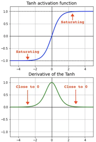
Thus if the pre-activation values lies in the saturating regions, then self.grad += (1-t²)*out.gradwill result into (1–1) = 0 * out.grad = 0. It has no gradient to propagate. Weights will not be updated effectively

NewWeight = OldWeight — learningrate * (derivitive of error w.r.t weight)

f(x) = 1 which is peak value. f’(x) will be 0.

A neuron is considered saturated when it reaches its peak value. At this point, the derivative of the parameter becomes zero, leading to no updates in the weights. This phenomenon is known as the Vanishing Gradient problem.

To address this, we should maintain pre-activations hpreact = embcat @ (W1) + b1 close to zero, especially during initialization. This can be achieved by scaling down W1 and b1.

# -------------------------- Initializations ------------------------
n_embd = 10                             # The dimensionality of the character embedding vectors
n_hidden = 200                          # The number of neurons in the hidden layers of the MLP
vocab_size = len(itos)

g = torch.Generator().manual_seed(2147483647)                         # for reproducibility
C = torch.randn((vocab_size, n_embd),                 generator=g)
W1 = torch.randn((n_embd*block_size, n_hidden),       generator=g) * 0.1
b1 = torch.randn(n_hidden,                            generator=g) * 0
W2 = torch.randn((n_hidden, vocab_size),              generator=g) * 0.1  # Scale down. Dont be confidentally wrong at initialization. 
b2 = torch.randn(vocab_size,                          generator=g) * 0

parameters = [C, W1, b1, W2, b2]
print(sum(p.nelement() for p in parameters))
for p in parameters:
    p.requires_grad = True

# -------------------------- Training Loop ------------------------
import torch.nn.functional as F
epochs = 200000
batch_size = 32
lossi = []
for epoch in range(epochs):
    ix = torch.randint(0, Xtrng.shape[0], (batch_size,), generator=g)
    Xb, Yb = Xtrng[ix], Ytrng[ix]       # batch X, Y

    # Forward pass
    emb = C[Xb]                           # embed the characters into vectors
    embcat = emb.view(emb.shape[0], -1)   # concatenate the vectors
    hpreact =embcat @ (W1) + b1           # hidden layer pre-activation
    h = torch.tanh(hpreact)               # Hidden layer
    logits = h @ (W2) + b2                # output layer
    loss = F.cross_entropy(logits, Yb)    # loss function

    # backward pass
    for p in parameters: p.grad = None
    loss.backward()

    # update
    lr = 0.1 if epoch < 100000 else 0.01 # step learning rate decay
    for p in parameters: p.data += -lr * p.grad

    # Track stats
    if epoch % 10000 == 0:
        lossi.append(loss.item())
        print(f'{epoch}: {loss.item():.4f}')
    lossi.append(loss.log10().item())
    break

The plot illustrates the distribution of ‘h’ values before and after scaling down, using 50 bins. After the scale down, It shows few ‘h’ values with |h| > 0.99.

plt.hist(h.view(-1).tolist(), 50)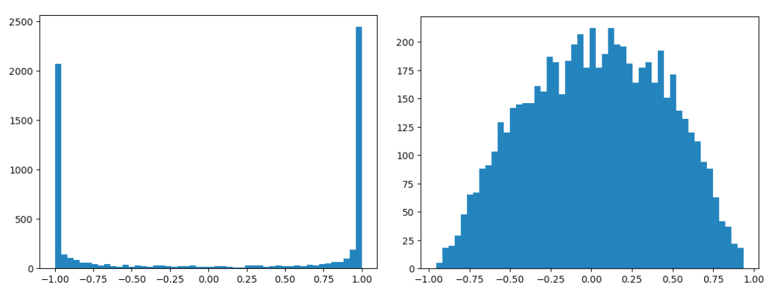

Distribution of ‘h’ values before (left) and after (right) scale down of W1 and b1.

The code below represents neurons with values less than -0.99 or greater than 0.99 as white dots.

# Show the neurons as white dot with value less than 0.99 or greater than 0.99. 
plt.figure(figsize=(20, 10))
plt.imshow(h.abs() > 0.99, cmap="gray", interpolation="nearest")
plt.xlabel("← tensor of length 200 →", labelpad=20, fontdict={"size":15})
plt.ylabel("← total 32 tensors →", labelpad=20, fontdict={"size":15});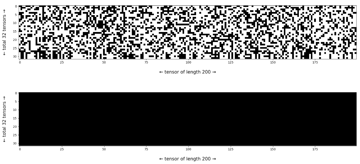

Number of neurons with with value less than 0.99 or greater than 0.99 are shown as white. After scale down (bottom), we dont have such neurons.

Batch Normalization

In order to avoid tanh saturation, we want our preactivation values to be roughly gaussian. Because if these are way too small numbers then the tanh will not be doing anything. If they are very large then tanh will be way too saturated, so gradients will not flow (dead neurons).

We will normalize the preacts to follow the standard deviation i.e zero mean and unit variance.

Calculate the Mean for each feature: For each feature , calculate the mean across all the examples in the mini-batch.

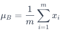
μB​ is the mean for the mini-batch, m is the number of examples in the mini-batch, and xi​ represents the value of the feature for the i-th example in the batch.

Calculate the Standard deviation: Standard deviation tells how spread out the values in a data set are around the mean (average).

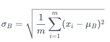
σB​ represents the standard deviation of the batch. xi​ are the individual data points in the batch. μB​ is the mean of the batch (for each feature). m is the number of samples in the mini-batch.

Normalize the feature: Normalize each feature value by subtracting the mean and dividing by the standard deviation

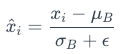
xi​ is the original value of the feature. μB​ is the mean of that feature in the mini-batch. σB​ is the standard deviation of that feature in the mini-batch. ϵ is a small constant to avoid division by zero.

... 
...
...
for epoch in range(epochs):
    ix = torch.randint(0, Xtrng.shape[0], (batch_size,), generator=g)
    Xb, Yb = Xtrng[ix], Ytrng[ix]       # batch X, Y

    # Forward pass
    emb = C[Xb]                           # embed the characters into vectors
    embcat = emb.view(emb.shape[0], -1)   # concatenate the vectors
    hpreact =embcat @ (W1) + b1           # hidden layer pre-activation
    # BatchNorm layer
    # -------------------------------------------------------------
    bnmeani = hpreact.mean(0, keepdim=True)
    bnstdi = hpreact.std(0, keepdim=True)
    hpreact = (hpreact - bnmeani) / bnstdi
    # -------------------------------------------------------------
    h = torch.tanh(hpreact)               # Hidden layer
    logits = h @ (W2) + b2                # output layer
    loss = F.cross_entropy(logits, Yb)    # loss function

...
...
...

Now we can train with above code. However, the issue is that we would not achieve a very good result because we want this to be roughly Gaussian but only at initialization. We don’t want the distribution to be permanently constrained to a Gaussian shape. Ideally, we would allow the neural network to adjust this distribution, making it more diffuse or sharper, or allowing some tanh neurons to become more or less responsive. We want the distribution to be dynamic, with backpropagation guiding its adjustments.

Therefore, in addition to standardizing the activations at any point in the network, it’s also necessary to introduce a ‘scale and shift’ component. This allows the model to undo the normalization if it determines that it’s better for the learning process.

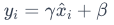
yi​ represents the final output of the batch normalization for the input xi​. The parameters γ and β are learned during training and allow the network to scale and shift the normalized data if needed.

... 
...
...
bngain = torch.ones((1, n_hidden))
bnbias = torch.ones((1, n_hidden))
for epoch in range(epochs):
    ix = torch.randint(0, Xtrng.shape[0], (batch_size,), generator=g)
    Xb, Yb = Xtrng[ix], Ytrng[ix]       # batch X, Y

    # Forward pass
    emb = C[Xb]                           # embed the characters into vectors
    embcat = emb.view(emb.shape[0], -1)   # concatenate the vectors
    hpreact =embcat @ (W1) + b1           # hidden layer pre-activation
    # BatchNorm layer
    # -------------------------------------------------------------
    bnmeani = hpreact.mean(0, keepdim=True)
    bnstdi = hpreact.std(0, keepdim=True)
    hpreact = bngain * ((hpreact - bnmeani) / bnstdi) + bnbias
    # -------------------------------------------------------------
    h = torch.tanh(hpreact)               # Hidden layer
    logits = h @ (W2) + b2                # output layer
    loss = F.cross_entropy(logits, Yb)    # loss function

...
...
...

That’s it for this blog. Thanks for the reading.

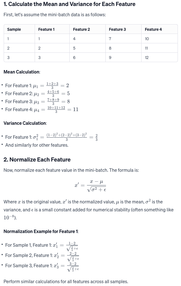
Appendix-A Batch normalization example