Fun with Freeform Receiver Design Using a Sound Card
How experimenting with wireless communication conventions using sound led to a surprising source of bit errors.
Fun with Freeform Receiver Design Using a Sound Card
How experimenting with wireless communication conventions using sound led to a surprising source of bit errors.

image by artist fiolisaviy
Introduction
There may be no usefulness for this, but I feel kind of “errrr” when people say with wireless communication: begin each packet with a known pattern and prevent runs of identical bits. Here, the goal is to poke at those conventions a little and see what breaks, what holds up, and what can be learned by sending data over ordinary audio gear between two locations with sound cards, a speaker and a microphone. Packets are still used, but without a start pattern to flag where a packet begins or to lock the receiver’s clock to bit transitions. Instead, packet location and timing are inferred from oversampling and a fixed packet length. The audio interface runs at a sample rate far higher than the symbol rate, so each bit spans many samples. With packets constrained to 256 bits, the receiver measures the captured duration and divides by 256 to get an initial bit period estimate, then refines that estimate while decoding. In effect, the packet is allowed to “land” anywhere inside a 256-bit-wide sampling net, and the clock transitions are fit after the fact.
Avoiding a preamble pushes the burden onto clock recovery, especially across long sequences of the same bit where no transitions are visible. Many systems prevent that by whitening (as in Bluetooth) or bit-stuffing (as in USB), ensuring frequent transitions that help a receiver track timing. Here the hope is that heavy oversampling and a fixed packet length soak up the uncertainty. A second assumption is that the transmitter’s clock does not wander too much over a 2.56-second packet and that both ends are crystal-disciplined so their absolute rates are close enough that a single bit width can be fit without continuous rescaling
A binary frequency-shift keying (FSK) scheme is used: one tone for zero and another for one, the same basic idea that carried data over dial-up phone lines, repurposed here for an open-air acoustic link through speakers and microphones.
FSK is friendly to the senses and to audio tooling. The binary tones can be heard and seen in both time and frequency plots. Figure 1 illustrates this using the free audio tool, Audacity. The time domain view in Fig. 1A helps eyeball symbol timing, the spectrum in Fig. 1B decodes the binary values indirectly through the tone frequencies of 1 kHz and 2 kHz. Fig. 1C computes the RMS energy in a signal-plus-noise window which can provide a rough estimate of a signal to noise ratio (SNR) when compared with a nearby noise-only window. FSK’s advantage here is not data capacity but visual debuggability which is invaluable when iterating quickly. A narrowband interferer will be visible as a horizontal line in the spectrum. A compressor will briefly flatten peaks in the time domain. A misaligned clock smears transitions in both plots. These clues are easy to capture and reason about in common audio tools.

Figure 1: Example of debugging in Audacity: bits and spectrum can be seen together for FSK. A) Time-domain view of symbols. B) Frequency spectrum with visible 1 kHz and 2 kHz components. C) RMS measurement for a signal-plus-noise window that can be compared with a noise-only window to approximate SNR.
The code that accompanies this article is in gnuradio-examples/analysis/test_clock_recovery (repository potto216/gnuradio-examples), primarily fsk_baseline.py and fsk_cli.py A discussion on the code generation is in the conclusion.
Waveform Design
Frequency was chosen over amplitude or phase because it tends to survive the audio chain in a state that can be decoded because it is relatively insensitive to amplitude changes¹. Level controls, automatic gain control, compressors, and soft clipping all reshape amplitude in level-dependent ways and often introduce new harmonics. Loudspeakers and microphones impose frequency-dependent amplitude and phase changes. Also, the sound-card sample-rate errors are typically on the order of tens to a few hundred parts per million, so an audio tone might drift by only a few hertz over a minute. In prior measurements of this setup (see Measuring the frequency distortion of my sound card with Fourier | by Paul Otto | Medium), frequency wander of roughly 1.5 Hz over a minute was observed, which is negligible relative to the 1 kHz tone spacing used in a packet lasting 2.5 seconds.
The binary zero is transmitted at f₀ = 1 kHz and the binary one at f₁ = 2 kHz. These are well inside a typical sound card’s passband and are spaced far apart compared with the expected hertz-level drift. Figure 2 relates the tones to the packet structure. The symbol rate is 1/T=100 symbols per second, so a 1 kHz tone contains 10 cycles per bit and a 2 kHz tone contains 20 cycles per bit. At a 44.1 kHz sample rate, each bit comprises 441 samples, which is ample resolution to fit timing after capture.
Packet generation is handled by build_tx_signal, which draws random bits and calls modulate_fsk. A short Hann taper (make_edge_taper) is applied at symbol boundaries to reduce spectral splatter from abrupt transitions. This tapers the edges without altering the bit centers where decisions are made, much like easing a car into and out of a lane change rather than yanking the wheel.

Figure 2: Diagram of a transmitted packet. A) The packet is 256 bits long and lasts 2.56 seconds. B) Bits are sent at 100 symbols per second. C) Each bit is either ten cycles at 1 kHz (zero) or twenty cycles at 2 kHz (one), with gentle edge tapering visible. D) The waveform is sampled at 44.1 kHz (44,100 samples per second).
Receiver Decoder Design
The receiver is divided into detection and demodulation.
Detection is implemented in detect_packet, which compares energy in the f₀ and f₁ bands against energy estimated from surrounding “noise” bands. Figure 3 sketches the idea. Guard bands around f₀ and f₁ are excluded when estimating noise to avoid bias from spectral leakage and sidelobes; a strong tone spills a little energy into adjacent bins and counting it as “noise” would dilute the contrast. DC is excluded as well because small offsets, mains hum, and slow drifts concentrate there and do not reflect the relevant noise background. A window of two symbol periods is used so the estimate is fast enough to follow changes but long enough to average down variance. Larger windows improve stability but react sluggishly when a packet begins; smaller windows respond quickly but fluctuate more. The chosen size is a compromise that works well with the symbol rate and tone spacing in this setup.

Figure 3: The detector compares energy at f₀ and f₁ with the rest of the band. A) Spectrogram with dotted red regions indicating guard bands excluded from the noise estimate and the DC region excluded at the bottom. Green lines mark f₀ and f₁. B) Time-domain signal with symbols labeled by their dominant tone.
Demodulation is performed by demodulate_from_start, which uses metric_for_tau to score candidate timing offsets. Conceptually, two narrow filters measure energy near f₀ and f₁; their difference forms a per-symbol decision variable. Because no preamble anchors timing, the entire packet is evaluated multiple times while sliding a candidate clock across it. The search runs in two stages. A coarse scan evaluates 16 evenly spaced phase positions within one symbol. Around the best coarse position, a fine search explores a small [−16, +16] sample window to pinpoint the optimum. Once timing is fixed, bit decisions compare the two filter energies over each symbol. This whole-packet approach is computationally heavier than symbol-by-symbol tracking, but it harvests the full integration gain of 256 symbols at once and is surprisingly robust when the SNR is high and clocks are close.

Figure 4: Packet-wise demodulation. A) The detector narrows the start to within a symbol. B) A coarse 16-position scan finds the best phase within the symbol. C) A fine, sample-by-sample search refines timing, after which decisions are made by comparing per-symbol energies.
Experiment
A single random 256-bit packet was transmitted repeatedly under three conditions. First, a wired loopback connected the sound card’s output to its input with a 3.5 mm TRS cable. This provides a best-case baseline. Second, a small Bose speaker transmitted to a headset microphone at a short, fixed distance; playback used Windows Media Player and recording used Audacity. Third, as shown in Figure 5 a Samsung monitor’s built-in speakers transmitted to the same headset microphone under similar geometry.

Figure 5 shows the over-the-air capture setup for the Samsung monitor; the Bose setup matched it closely.
Multiple packets were recorded in each configuration and analyzed. A packet from each setup is shown in Figure 6. In the wired loopback, the envelopes of the 1 kHz and 2 kHz symbols are similar in height over the first ten bits. For the Bose speaker, the 2 kHz tone tends to be stronger than the 1 kHz tone, suggesting a high-pass characteristic from the acoustic chain. With the Samsung monitor, the trend reverses: the higher frequency is attenuated more. Because the same microphone was used in both over-the-air captures, the opposing trends point to differences in the speakers rather than the mic.

Figure 6: Comparing received packets across wired loopback and two speakers. Yellow arrows highlight that the Bose capture emphasizes 2 kHz relative to 1 kHz, while the Samsung capture does the opposite.
Ambient noise levels tell a complementary story. Figure 7 compares RMS values from noise-only segments. The two over-the-air captures cluster around −30 decibels relative to full scale (dBFS), while the loopback sits near the system floor around −100 dBFS, comparable to the 16-bit theoretical limit of about −96 dBFS so likely constrained by the sound card’s own noise. This suggests the observed noise in the speaker captures is dominated by the microphone not the digital path.

Figure 7: Ambient noise comparison using RMS. Over-the-air captures are around −30 dBFS; the wired loopback is near the device floor.
Looking closely at individual bit symbols in Figure 8 shows the spectral fingerprints of the three paths for the zero and one symbols. The loopback shows matched amplitudes as expected. The Bose and Samsung traces invert that relationship, consistent with their opposite frequency responses. The Samsung example shows additional envelope fluctuations within a symbol — evidence of amplitude modulation from resonances or dynamic processing in the speaker path.

Figure 8: Zero- and one-symbol comparisons for loopback, Bose, and Samsung captures. The speakers invert the relative amplitudes; the Samsung trace shows extra modulation within a symbol.
Because the SNR was high in all conditions the demodulator usually produced error-free decisions. When errors appeared, they were not random bit flips from noise but structural issues: local time shifts or inserted distortions that misaligned symbol boundaries.
Figure 9 contrasts two Samsung packets: packet 3 decodes cleanly while packet 4 does not. The errors are consistent with dropped audio — if a short segment around bit indices 186–188 from packet 3 is excised, the remainder aligns with packet 4, and the subsequent symbol boundaries shift. Many error-control codes assume substitution errors, not deletions; a few tens of milliseconds of lost audio at a 100 Hz symbol rate force a misparse that standard error correction will not correct.

Figure 9: Comparison of two packets from the Samsung setup. Packet-length alignment suggests a short audio drop in packet 4, producing a persistent symbol offset.
Figure 10 shows a different failure mode when comparing loopback and Bose captures. The highlighted regions exhibit periodic, nonlinear distortions whose waveforms do not match either 1 kHz or 2 kHz. The effect is to nudge effective symbol timing to cause intermittent decision errors. Such artifacts are typical of consumer audio processing — AGC, compressors, limiters, or “enhancement” features — that momentarily alter amplitude and introduce harmonics, especially around transients.

Figure 10: Bit transmission errors for the loopback and Bose speaker. Distortions indicated by the magenta arrows are from inserted energy and shift symbols out of alignment with frequencies unrelated to f₀ and f₁ causing bit errors.
Conclusion
I didn’t expect the most interesting find. Bit failures were caused by the digital audio pipeline misbehaving: either sample dropouts or inserted bursts — both slide symbol timing far from the receiver’s expectation. Once timing slides, decisions stay wrong for the rest of the packet. The root cause of this slide is probably underruns/overruns in the audio stack or OS scheduling hiccups.
Excluding the pipeline induced errors the method of sending a fixed size packet without a header worked in a high SNR environment. A detector that watches for sustained tone energy, coupled with heavy oversampling and a fixed 256-bit window, allowed packet-wise timing fits without a preamble. Stable sound-card clocks kept drift small over 2.56 seconds, and whole-packet integration delivered robust decisions when the pipeline behaved. The cost is high computation from both oversampling and the coarse-to-fine search which effectively demodulates the packet multiple times. The second issue’s burden can be eased with FFT-based filter banks, polyphase resampling for fractional delays, and a decision-directed timing loop once a coarse lock is found. Narrowing filters adaptively around f₀ and f₁ after detection can reduce per-symbol cost.
The code for this article gnuradio-examples/analysis/test_clock_recovery, was generated using ChatGPT 5 Thinking based on the set of requirements I iterated on with ChatGPT in code_requirements_prompt.txt. I found the suggestions it provided in the requirements iteration phase very helpful especially on pointing out issues I had not considered. Also, I found its initial code (basically the first commit) accurate to the requirements. I think its performance is a testament to the quality of the signal processing and communications material available for its training and the ability of commercial large language models to shape next phrase prediction into useful output.
The next steps are:
- Measure bit errors at lower SNR to map out margins and to quantify the impact of room reflections and intersymbol interference.
- Use soft-decision decoding with a simple trellis code and a Viterbi decoder to measure bit error rate improvement.
- Analyze the detector algorithm to determine what its scaling parameter should be to cover a wide range of SNR.
- Automate the plot alignment by carrying timing estimates through the visualization pipeline rather than hand-tweaking offsets.
- Determine the symbol taper’s benefit when adjacent bits repeat. If symbols are identical, edge tapering sheds energy that could have contributed to the decision without reducing splatter.
- Determine the source of the audio pipeline induced errors.
Tossing out the preamble did not doom the link. With generous oversampling, a fixed-length packet, and whole-packet timing search, the FSK signal was decoded without error (excluding audio pipeline errors). This will change in future articles where the SNR will decrease and noise, interference, and intersymbol interference from reflections will have an impact.
Notes
¹FSK is insensitive to amplitude and phase changes as long as their rate of change is not a significant fraction of the FSK frequency or the spacing between tones.
The writing process used ChatGPT 5 (Extended Thinking)
메타데이터
- post_id
- eb7fcf1d3aad
- slug
- fun-with-freeform-receiver-design-using-a-sound-card-eb7fcf1d3aad
- url
- https://medium.com/@potto_94870/fun-with-freeform-receiver-design-using-a-sound-card-eb7fcf1d3aad
- canonical_url
- https://medium.com/@potto_94870/fun-with-freeform-receiver-design-using-a-sound-card-eb7fcf1d3aad
- author_url
- https://medium.com/@potto_94870
- status
- ok
- fetched_at
- 2026-06-22 00:13:37