Assessing and Comparing Classifier Performance with ROC Curves in Python for Financial Analysis

This article shows how to use ROC curves and AUC in Python to rigorously evaluate, compare, and threshold-tune financial classifiers so model choices align with real economic trade-offs between false positives and false negatives.

Download link:

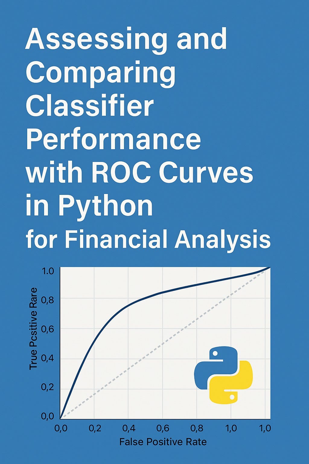
[embed]Assessing and Comparing Classifier Performance with ROC Curves in Python for Financial Analysis This article shows how to use ROC curves and AUC in Python to rigorously evaluate, compare, and threshold-tune…nilimesh.substack.com

[embed]From Data to Insights: Advanced Analytics, Machine Learning & Data Science Transform raw data into actionable intelligence. Our data into actionable intelligence articles (with codes) offer…advanceddataanalysis.gumroad.com

Article Outline:

1. Introduction — Why classifier evaluation matters in finance (credit risk, fraud detection, churn, AML) and why accuracy alone can mislead when costs are asymmetric and classes are imbalanced.
2. ROC Curve Essentials — Defining True Positive Rate (sensitivity/recall) and False Positive Rate (1–specificity); how varying thresholds traces the ROC; interpreting the random baseline vs. the ideal top-left corner.
3. AUC (Area Under the ROC Curve) — What AUC measures as threshold-independent ranking quality; practical interpretation for finance teams and model risk committees.
4. Financial Costs and Thresholds — Mapping false positives/negatives to dollars (e.g., missed fraud vs. unnecessary declines); translating ROC positions into expected loss and business KPIs.
5. Python Environment Setup — Libraries for an applied workflow: scikit-learn (models, ROC/AUC), numpy/pandas (data), matplotlib/seaborn (plots).
6. Problem Framing & Data Schema — Typical financial features (transaction behavior, credit bureau attributes, account tenure); target definition (e.g., default or fraud).
7. Model Training Portfolio — Training Logistic Regression (interpretable baseline), Random Forest (nonlinear patterns), and SVM/Gradient Boosting (strong benchmarks) with probability outputs.
8. ROC Construction in Python — Computing roc_curve, plotting multiple models on one chart, and annotating AUC; visual checks for dominance and crossings.
9. Choosing Operating Points — Selecting thresholds via Youden’s J, maximizing expected utility, or meeting regulatory constraints (e.g., fixed FPR); converting choices to confusion matrices and business impact.
10. Beyond ROC for Finance — When Precision–Recall curves are preferable (rare-event fraud), calibration checks (reliability plots), and cost-sensitive evaluation.
11. Robust Validation — Train/validation/test splits, cross-validation, leakage prevention, reproducibility; aggregating ROC/AUC across folds and segments (customer cohorts).
12. End-to-End Python Walkthrough — Complete example: data generation → model fitting → ROC/AUC comparison → threshold selection → interpretation for financial KPIs.
13. Common Pitfalls & Best Practices — Handling extreme imbalance, aligning metrics with policy rules, documenting decisions for audits and model risk governance.
14. Conclusion & Next Steps — Embedding ROC analysis in production model monitoring, drift checks, and cost-aware re-thresholding.

12. End-to-End Python Walkthrough

import numpy as np
import pandas as pd
import matplotlib.pyplot as plt
import seaborn as sns
from sklearn.datasets import make_classification
from sklearn.model_selection import train_test_split
from sklearn.linear_model import LogisticRegression
from sklearn.ensemble import RandomForestClassifier
from sklearn.svm import SVC
from sklearn.metrics import roc_curve, roc_auc_score

# Data simulation
X, y = make_classification(n_samples=2000, n_features=20, n_informative=10,
                           n_redundant=5, n_classes=2, random_state=42)
X_train, X_test, y_train, y_test = train_test_split(X, y, test_size=0.3, random_state=42)

# Models
log_reg = LogisticRegression(max_iter=1000)
rf = RandomForestClassifier(n_estimators=100, random_state=42)
svm = SVC(probability=True, random_state=42)

log_reg.fit(X_train, y_train)
rf.fit(X_train, y_train)
svm.fit(X_train, y_train)

# Probabilities
y_prob_log = log_reg.predict_proba(X_test)[:,1]
y_prob_rf = rf.predict_proba(X_test)[:,1]
y_prob_svm = svm.predict_proba(X_test)[:,1]

# ROC
fpr_log, tpr_log, thresholds_log = roc_curve(y_test, y_prob_log)
fpr_rf, tpr_rf, thresholds_rf = roc_curve(y_test, y_prob_rf)
fpr_svm, tpr_svm, thresholds_svm = roc_curve(y_test, y_prob_svm)

# AUC
auc_log = roc_auc_score(y_test, y_prob_log)
auc_rf = roc_auc_score(y_test, y_prob_rf)
auc_svm = roc_auc_score(y_test, y_prob_svm)

# Plot
plt.figure(figsize=(8,6))
sns.set_style("whitegrid")
plt.plot(fpr_log, tpr_log, label=f"Logistic Regression (AUC={auc_log:.2f})")
plt.plot(fpr_rf, tpr_rf, label=f"Random Forest (AUC={auc_rf:.2f})")
plt.plot(fpr_svm, tpr_svm, label=f"SVM (AUC={auc_svm:.2f})")
plt.plot([0,1],[0,1],'k--')
plt.xlabel("False Positive Rate")
plt.ylabel("True Positive Rate")
plt.title("ROC Curves for Financial Classifiers")
plt.legend()
plt.show()

# Best Threshold (example for Logistic Regression)
j_scores = tpr_log - fpr_log
j_best_index = np.argmax(j_scores)
print("Best Threshold (Youden's J):", thresholds_log[j_best_index])