Machine Learning Series (Part 30) : From Overfitting to Generalization — Understanding Ridge Regularization

In our last blog, we learned the learning curves of different polynomial fit. The 4th degree polynomial was overfitting the data points as the validation error was higher than the train error. This model performed well in training by capturing all the data points, but when provided with unseen data in the validation, the performance was poor. There should be a way to reduce the model becoming complex and learning every data point? In order to handle this scenario, we have a strategy called ‘regularization’.

Let’s say we prepare paneer butter masala which is mostly a likeable dish for all. Unfortunately, it becomes too spicy. To reduce the spiciness, we add butter or fresh cream or a table spoon of sugar. Once the dish is prepared, we may not be able to remove the added spice of the dish as it would have blended well, but we were able to constrain the spice level by adding the other ingredients. This is how the role of regularization behaves in machine learning as well. When a model is overfitting, regularization adds a penalty term to the loss function to constrain the model complexity. We will clearly see how this process takes place.

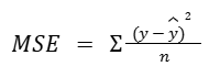
The loss function for a linear model is the average of the sum of squared difference between the predicted and the actual value. It is represented as:

To this mean squared error, we add a penalty term. The penalty term added is:

Let’s see in depth how adding this penalty term reduces the loss function. Here is a walkthrough with the examples.

Assume there are two data points (0,1) and (4,9). Plotting these data points look as below:

Now, what happens if we train a linear model with these points as training data. With only two training points, the model can fit the training data perfectly. And in our case it has got overfit. However, such a model may not generalize well to new unseen data.

The loss error for the training data is zero as the actual and predicted values are the same! We know that,

For the first data points (0,1) and (4,9) we shall do the live error calculation:

Basically, y = mx + c

We do not know the values of ‘m’ which is the slope and the ‘c’ which is the intercept.

As already seen, m is calculated by change in rise divided by change in run.

i.e ,

With our two data points (0,1) and (4,9) we can calculate the slope m.

So the slope is 2 units. Having found slope, we can easily calculate the intercept by substituting in the y = mx + c equation.

Let’s take any x and y values from the two data points. For now we can take 1 from the (0,1) data point.

1 = 2(0) + c

So c=1, it is going to remain the same as the intercept is a constant. From the calculated slope and intercept values, the y hat will be calculated. It is very clear that the actual values and the predicted values are exactly the same and we knew that as well, but I wanted to perform the error calculation lively so that it is more reachable.

The below tabular format shows the actual y (i.e y value from the data points) , the predicted y and the squared error.

The squared error for each of the two data points is 0, and obviously the sum and mean of them will be 0.

When we test this model with new data points, the test error is prone to be high as we all know that an overfitting model will not be able to generalize the unseen data points. Let’s plot some points as test data.

From the line of fit, we understand that the model has not generalized well. Let’s try to calculate the error for the test data the same as we did for error calculation for training data.

From the above calculation we can see that the errors are too high while in training the error was completely 0 indicating a clear overfit model. Now, the average of the above errors would be:

As the error during testing is so high, we might not be in a position to reduce the error by means of adding extra data points and re-training it. That is why regularization’s role enters. Through regularization we add a penalty to the error function. In the start of the blog we saw that the penalty term being added is

Theta represents the model parameters, that is the values for the attributes of the dataset used in the predictive equation, it is the weight of the attribute. The intercept is usually represented by

While the remaining theta values

correspond to the coefficients of the features (aka attributes).

In short, theta represents the coefficients (weights) learned by the model for each feature. For example, in the California house price prediction, we have area, no. of rooms, distance from the ocean — So for each of these features, a penalty is added. In the penalty we have squared the co-efficients and added it to the MSE. Since the penalty uses the square of the coefficients, it is called an L2 penalty. The overall technique of adding this L2 penalty to the loss function is known as Ridge Regularization. You might wonder what L1 means — we will explore that in the next part.

When L2 regularization is applied to a linear regression model, it is commonly referred to as Ridge Regression. People often use the terms ‘ridge regularization’ and ‘ridge regression’ interchangeably, but remember that ridge regularization refers to the regularization technique itself while ridge regression is when L2 is applied to linear regression.

What happens in ridge regression is, during the training the ridge regression forces the model to choose slope value such that the model does not use large slope values and is more likely to generalize well to unseen data.

During the training the MSE is calculated, along with it the penalty per feature is squared and added to the MSE. In our example, there is only one predictor variable — year of business , hence there would be one penalty term getting added. Let’s say we keep the theta value as 1.2 and alpha (hyperparameter) as 10 for our case. This makes the model to reduce the slope from m=2 to a lower value. What really happens is, the model accepts an extra amount of training error but reduces the slope value. Due to this, the training error will be high but the test error decreases.

Image Courtesy : Gemini

We all know that, in a linear regression, the model tries to fit the best fit of line in the data points. This represents the most suitable slope and intercept value to those data points. In ridge regression, during the training as we add a penalty term to the loss function, the model tries to adjust the slope value to make the model less likely to overfit the training data.

Adding the penalty to the error in the training becomes becomes as below:

We saw that the MSE during the training was 0. So now let’s add the penalty to this as the formula goes by

Does the penalty term make you feel dizzy?! Let me clarify. We had just seen that the theta presents each of the attributes. So if there are m number of attributes, then for each of them, a theta value is decided, squared and summed up together. Then finally it is multiplied by the alpha. In our case we only have year of business. Hence we can remove the sigma. So the equation becomes

If we substitute the values, it becomes:

As we can see, the MSE is 0 but after adding the penalty term, the overall loss function becomes larger. So at this stage, the model adjusts the slope value typically like “Omg, the error is too high, let me simplify the parameter” i.e the model notices that the overall cost has increased because a large slope value is being penalized, it starts shrinking the slope. And this happens via the process of gradient descent which is clearly explained end to end in part 27.

For simplicity, we are assuming that after a few gradient descent updates, the slope decreases from 2 to 1.5. The exact value is not important here; the key idea is that ridge regression encourages smaller parameter values.

the new equation for the fit becomes y = 1.5x + c

For this equation, the predicted value becomes as

The MSE for the line of fit y = 1.5x + c is:

Now let’s add the penalty to this.

You might wonder, the MSE itself is 0, why do we add the penalty and make it 14.4 and similarly in the second time, the slope value got changed to 1.5 but here as well the training error became more than the previous error which is 16.4

Your doubt is valid. While adding the penalty to the training error has increased the error, it plays a significant role in the testing data which we shall see now.

Let’s calculate the error for the test data based on the new slope value which got changed in the ridge regression.

Now if we calculate the MSE for this data, it becomes

As we can see, the slope value of the ridge regression line has drastically reduced the test error. Though the training error was high when we added the penalty, it has adjusted the slope value to become less sensitive to the training data. As a result, the model often performs better on unseen test data. Whereas the test error without the penalty ( i.e normal linear regression) had 14.4 as test error. What the ridge regression does is that it shrinks the co-efficients to close to 0. In our example, shrinking the coefficient means reducing the slope value.

The change of slope value happens via the gradient descent.

Note: For a complete end to end understanding of gradient descent along with a numerical walkthrough, kindly refer to part 27 of this series.

For now, we can just try to comprehend that adding the penalty to the MSE makes the model adjust the parameters to reduce overfitting and improve generalization.

In the next part, we shall see about the other two types of regularization which is the LASSO and Elastic Net.