Stars, Galaxies, and Quasars: A Machine Learning Approach to Stellar Classification (MLflow…
As children, many of us have gazed up at the starry sky. We had so many questions about the universe like “What lies beyond?”, “Could there…
Stars, Galaxies, and Quasars: A Machine Learning Approach to Stellar Classification (MLflow, DagsHub)
As children, many of us have gazed up at the starry sky. We had so many questions about the universe like “What lies beyond?”, “Could there be an edge of the Universe? (I used to think that there is an edge of the universe like a giant cliff)”, “What came before the Universe?” and so on. While not all of us grew up to become astronomers, our deep-rooted curiosity about the remains universal.

Background Information for Project
Astronomy: humanity’s oldest science.
Astronomy is the scientific study of the universe and of the objects that exist naturally in space. It uses principles of physics, mathematics, and chemistry to help us understand the origins, evolution, and behavior of stars, planets, galaxies, and other cosmic phenomena.
Stars, Quasars, and Galaxies
Stars, galaxies, and quasars are the three important stellar objects in astronomy. They are the fundamental building blocks of the universe.
- Stars are massive luminous spheroids of plasma undergoing nuclear fusion and this process generates enormous amounts of energy, making them shine. They come in various types, sizes, and life cycles, from red dwarfs to explosive supernovae. Our own “Sun” is a yellow dwarf star.
- Galaxies are massive systems of stars, gas, dust, and dark matter bound together by gravity. They range from elegant spiral shapes, like our Milky Way, to colossal elliptical galaxies and irregular formations. Each galaxy is a cosmic metropolis housing millions to trillions of stars.
- Quasars or Quasi-Stellar-Objects (QSO) are at the center of some distant galaxies. They derive their name from their initial starlike appearance when discovered in the late 1950s and early 1960s. It is a supermassive black hole that is growing rapidly by gorging on huge amounts of gas and they are extremely luminous. The most powerful quasars have luminosities thousands of times greater than that of a galaxy such as the Milky Way.
The Challenge of Classification
However, classifying these objects-— stars, galaxies, and quasars is challenging. Due to factors like their varying distances, brightness, and positions in the vast expanse of space, they often appear as nearly indistinguishable smudges or dots of light in photometric data recorded by telescopes. Without precise analysis, distinguishing between these objects can be difficult.
A Machine Learning for Stellar Classification
To overcome these challenges, we use machine learning to classify stars, galaxies, and quasars.
Dataset Details
The data is from the Sloan Digital Sky Survey (SDSS).
- The SDSS provides an extensive dataset of photometric and spectroscopic data for celestial objects.
- Size: Over 1,00,000 labeled entries are categorized into stars, galaxies, and quasars.
- Every observation is described by 17 feature columns and 1 class column which identifies it to be either a star, galaxy, or quasar.
Features in the dataset
obj_ID= Object Identifier, the unique value that identifies the object in the image catalog used by the CAS.alpha= Right Ascension angle (at J2000 epoch).delta= Declination angle (at J2000 epoch).u= Ultraviolet filter in the photometric system.g= Green filter in the photometric system.r= Red filter in the photometric system.i= Near Infrared filter in the photometric system.z= Infrared filter in the photometric system.run_ID= Run Number used to identify the specific scan.rereun_ID= Rerun Number to specify how the image was processed.cam_col= Camera column to identify the scanline within the run.field_ID= Field number to identify each field.spec_obj_ID= Unique ID used for optical spectroscopic objects (this means that 2 different observations with the samespec_obj_IDmust share the output class).class= Object class (galaxy, star, or quasar object).redshift= Redshift value based on the increase in wavelength.plate= Plate ID, identifies each plate in SDSS.MJD= Modified Julian Date, used to indicate when a given piece of SDSS data was taken.fiber_ID= Fiber ID identifies the fiber that pointed the light at the focal plane in each observation.
How I Approached This Project
Building a robust machine learning pipeline requires a systematic approach to handle data preparation, model training, and evaluation.
Before that, I did some initial exploring in ipython notebook, you can find it here: Eda.ipynb.
Project Components
1. Data Ingestion
This stage ensures the availability of the dataset required for the pipeline. For this project, the dataset is stored in a dedicated GitHub repository. The steps involved are:
- Downloading the Dataset: The dataset is fetched from a remote URL if it doesn’t already exist locally.
- Extracting Data: The compressed dataset is extracted into a predefined directory, ensuring the data is ready for validation and further processing.
2. Data Validation
In this stage, the data is cleaned and validated against a predefined schema to ensure consistency and reliability. Key steps include:
- Loading Data: The data is read into a DataFrame for analysis.
- Dropping Unnecessary Columns: Some columns in the original dataset contained identifiers or metadata that did not contribute to the classification task. These included:
**-> **obj_ID: Object identifier, unique to each observation but irrelevant for classification.
**->**spec_obj_ID: Spectroscopic object identifier, redundant for the task.
**-> **rerun_ID, run_ID, cam_col, field_ID: Metadata related to the imaging scan.
**-> **plate, MJD, fiber_ID: Related to observation instrumentation rather than celestial object properties.
**-> **alpha and delta: Astronomical coordinates, unnecessary for classification given the photometric data available.
After removing these columns we are left with features like redshift, photometric magnitudes (u, g, r, i, z), and the class label.
-
Schema Validation: The data is checked against a schema to ensure all required columns exist and adhere to expected data types.
-
Cleaning Data: Missing values and outliers are handled appropriately.
- Replaced placeholder values like
-9999.0withNaNto standardize missing data handling.
- Saving Cleaned Data: The validated and cleaned data is stored for the next stage.
3. Data Transformation
This stage prepares the data for model training by addressing issues like class imbalance, feature engineering, and normalization. The workflow includes:
- Train-Test Split: The data is split into training (75%) and testing (25%) subsets.
- Class Imbalance Handling: SMOTE is applied to balance the classes in the training set.
- Feature Engineering: Magnitude differences between photometric bands (
u_g,g_r,r_i,i_z) are computed to enhance feature representation. - Normalization: Numerical features are scaled using MinMaxScaler to ensure uniformity.
- Saving Transformed Data: The processed training and testing datasets are saved for use in model training.
Model Trainer
In this stage, machine learning models are trained and tuned using the processed data.
- Loading Transformed Data: The transformed and normalized training data is loaded for training.
- Model Selection and Training: Models like RandomForest, LightGBM, and XGBoost are trained with hyperparameter tuning.
- Hyperopt is used for hyperparameter tuning
- Tracking Experiments: Utilized MLflow for experiment tracking and reproducibility:
- Metrics Logged: Training and test accuracy.
Model Evaluation
The final stage evaluates the trained models on unseen test data. Key metrics are calculated to assess model performance, and the best model is selected for deployment. Steps include:
- Loading Test Data: The test dataset is loaded for evaluation.
- Performance Metrics: Computes classification metrics like accuracy, precision, recall, and F1-score.
This modular and systematic approach ensures the pipeline is efficient, maintainable, and adaptable to future changes or additional requirements.
Feature Engineering: Retaining Original Features and Magnitude Differences
In the data transformation stage, one critical decision was to retain both the original magnitude features (u, g, r, i, z) and the derived magnitude differences (u_g, g_r, r_i, i_z). Here’s why this approach is beneficial for the Stellar Classification task:
1. Preservation of Original Information
The original features represent absolute magnitudes in specific bands, such as ultraviolet (u), green (g), and infrared (i). These features directly correlate with physical properties of stars, such as their brightness and temperature. Removing them would mean losing critical information needed for accurate classification.
2. Complementary Nature of Magnitude Differences
Magnitude differences are derived features that highlight the relative changes between bands, effectively capturing color gradients and spectral properties. For instance:
u_gmeasures the difference between ultraviolet and green bands.g_rrepresents the gradient between green and red bands.
These relative measurements are essential for identifying specific star types based on their spectral energy distribution.
3. Enhancing Model Performance
The model is equipped with a richer feature space by retaining both absolute and relative features. This allows the algorithm to explore complex relationships and patterns in the data, improving classification accuracy.
Leveraging DagsHub for Efficient Project Management
For the Stellar Classification project, we utilized DagsHub, a powerful platform designed to manage data science and machine learning projects. It integrates seamlessly with tools like Git, MLflow, and DVC, enabling effective version control, experiment tracking, and collaboration. Here’s how DagsHub streamlined our workflow:
- Git Integration
- We hosted our project repository on DagsHub, leveraging Git for version control.
- Every change in code, configuration files, and documentation was tracked, making it easy to revert or collaborate.
2. MLflow Tracking
- MLflow experiments were tracked directly in DagsHub.
- Key metrics, hyperparameters, and artifacts (like trained models) were logged automatically during model training.
- The visual dashboard provided insights into experiment results and facilitated easy comparisons.
- We tracked experiments for RandomForest, XGBoost, and LightGBM with different hyperparameter configurations using MLflow.
- Each experiment’s results were logged and visualized on DagsHub, allowing us to identify the best-performing model.
Confusion Matrix Analysis
The confusion matrix reveals the model’s classification performance across the three classes: Galaxy, QSO (Quasar), and Star.

confusion matrix
Key Observations:
- Galaxy Class:
- Correctly classified: 14,569 (True Positives).
- Misclassified as QSO: 155, as Star: 153 (False Negatives).
- The model excels in identifying galaxies.
2. QSO Class:
- Correctly classified: 4,279.
- Misclassified as Galaxy: 517, as Star: 1.
- There is room for improvement in distinguishing QSOs from galaxies due to overlapping features.
3. Star Class:
- Correctly classified: 5,323.
- Rare misclassification (3 as Galaxy)
Github link.
Dagshub Experiments link.
References
Dataset reference
- fedesoriano. (January 2022). Stellar Classification Dataset — SDSS17. Retrieved [Date Retrieved] from https://www.kaggle.com/fedesoriano/stellar-classification-dataset-sdss17.
- The data released by the SDSS is under public domain. Its taken from the current data release RD17. More information about the license: http://www.sdss.org/science/image-gallery/
메타데이터
- post_id
- ee09f5cdb997
- slug
- classifying-the-cosmos-a-stellar-classification-machine-learning-project-ee09f5cdb997
- url
- https://medium.com/@kavyasree42/classifying-the-cosmos-a-stellar-classification-machine-learning-project-ee09f5cdb997
- canonical_url
- https://medium.com/@kavyasree42/classifying-the-cosmos-a-stellar-classification-machine-learning-project-ee09f5cdb997
- author_url
- https://medium.com/@kavyasree42
- status
- ok
- fetched_at
- 2026-08-27 15:43:20