How to estimate flexibility of FPGA interconnect architecture?

Estimating the flexibility of an FPGA’s interconnect architecture is a complex, multi-faceted problem that sits at the heart of FPGA architecture research. There’s no single “flexibility number,” but rather a set of metrics and methodologies used to quantify it.

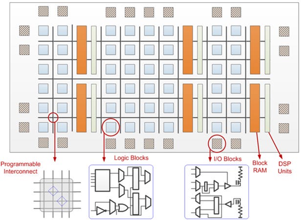
Here’s a structured approach to estimate FPGA interconnect flexibility, from high-level concepts to specific, measurable metrics.

1. Understanding Interconnect “Flexibility”

First, define what “flexibility” means in this context. It generally encompasses:

• Routability: The ability to successfully connect a wide variety of circuit netlists.
• Predictability: The likelihood that a circuit will route successfully without requiring exotic, hard-to-find routing paths.
• Performance: The ability to provide low-delay paths between commonly connected logic blocks.
• Efficiency: The trade-off between flexibility and the overhead (area, delay, power) it introduces.

2. Key Architectural Metrics for Quantitative Estimation

These are the concrete, measurable properties of the interconnect that you can extract from architecture documents or CAD tool reports.

A. Connectivity Metrics

These measure “how many connections are possible.”

1. Fanout (Fc): The number of wire segments a logic block pin or a routing track can connect to.

• Fc_in: Number of routing tracks a Logic Block (CLB) input pin can connect to. High Fc_in improves routability.
• Fc_out: Number of routing tracks a Logic Block (CLB) output pin can connect to. High Fc_out helps with “sourcing” signals.
• You want a balance. Very high Fc increases flexibility but also significantly increases parasitic capacitance and area of the routing multiplexers.

2. Switch Block Flexibility (Fs): This defines how routing tracks can be connected to each other at the intersections of the horizontal and vertical channels.

• Fs = 3 (Wilton Scheme): A track can connect to one track in each of the three other directions (left, right, and the opposite track on the perpendicular channel). This is a common, well-balanced design.
• Fs = 2 (Disjoint): Simpler, less flexible.
• Higher Fs: More flexible but more switches (area/power cost). You can analyze the switch block topology (e.g., subset, universal, Wilton) for a deeper understanding.

3. Connection Block Flexibility: Similar to Fc, but specifically describing the mux that connects logic block pins to the routing tracks.

B. Topology and Length Distribution Metrics

This measures “what kinds of connections are possible.”

1. Wire Segment Length Distribution: The mix of wire segments of different lengths.

• Length-1 Wires: Connect only to adjacent switch blocks. Highly flexible for local connections but high delay for long-distance.
• Length-4 Wires: Span 4 logic blocks before hitting a switch block. Excellent for low-delay medium-range connections, but less flexible for local routing.
• Half-length and Full-length Wires: Span half or the entire chip. Critical for global signals (e.g., clocks, resets) and low-skew long-distance paths.
• A flexible architecture has a balanced mix of these lengths. A predominance of length-1 wires is very flexible but slow. A predominance of long wires is fast but can lead to routing congestion.

2. Routing Hierarchy: The presence of dedicated, low-flexibility but high-performance interconnect for specific purposes.

• Dedicated Carry Chains: Fast adders.
• Direct Links: Neighbor-to-neighbor connections between adjacent CLBs, bypassing the general routing.
• Dedicated Clock Trees: Low-skew, high-fanout networks.
• While not “flexible” themselves, these dedicated networks free up the general-purpose interconnect for other tasks, effectively increasing its available flexibility for random logic.

3. Practical Methods for Estimation

You don’t always have access to the transistor-level layout. Here’s how to estimate flexibility in practice.

Method 1: Using Vendor Datasheets & Architecture Docs

Look for the following in documents like Xilinx’s “Architecture” or Intel’s “Configuration Handbooks”:

• Maximum Logic Utilization: Vendors often state a realistic maximum (e.g., 85–90%). A higher achievable utilization suggests a more flexible interconnect, as it can handle denser packing.
• Routing Resources Description: They often describe the ratio of long/longer lines to direct interconnect. A more diverse set indicates better flexibility for different connection needs.
• Switch Matrix Description: How the routing channels connect. Look for terms like “high-performance switch matrix.”

Method 2: The Benchmarking & CAD Flow (Most Accurate)

This is the academic and industrial standard. The process is:

1. Select Benchmark Circuits: A large and diverse set of standard benchmarks (e.g., from the MCNC or VTR benchmark suites). This includes circuits of different sizes and structures (arithmetic, control logic, DSP, memory-based).
2. Use an FPGA CAD Flow:

• Synthesis & Technology Mapping: Convert RTL into LUTs and FFs.
• Packing: Pack LUTs and FFs into Complex Logic Blocks (CLBs).
• Placement: Assign CLBs to specific locations on the FPGA grid.
• Routing: This is the critical step. Use a detailed router (like the one in the VTR project).

3. Analyze the Results: The key metrics from this flow are:

Method 3: The “Stress Test” with Your Own Designs

If you have the FPGA in hand, you can perform empirical tests:

1. The Utilization Sweep: Take a design and gradually increase its logic density. Note the point at which the router starts to fail or when timing closure becomes impossible. A more flexible architecture will allow for higher utilization before breaking down.
2. The “Pathological” Test: Create a circuit with a very non-local, high-fanout routing demand (e.g., a cross-chip bus or a shuffling network). See how well it routes in terms of timing and resource usage compared to a more localized design.

Summary: A Practical Estimation Checklist

To quickly estimate the flexibility of an FPGA’s interconnect, ask these questions:

1. What is the mix of wire lengths? (Look for a balance of short, medium, and long).
2. What is the switch block flexibility (Fs)? (Higher is generally more flexible).
3. What is the pin connectivity (Fc)? (Balanced Fc_in and Fc_out is good).
4. Are there abundant dedicated resources? (Carry chains, direct links, etc.) These improve effective flexibility.
5. What is the minimum channel width (W_min) required for a standard benchmark suite? (This is the gold-standard metric).
6. How high can logic utilization go before routing fails? (Higher is better).

For modern FPGAs (Xilinx/AMD UltraScale+, Intel Agilex), the interconnect is highly optimized and very flexible, but this comes at the cost of immense complexity. The best way to “feel” the difference is to take a very dense design and try to route it on a smaller, older FPGA family versus a larger, modern one. The modern architecture will typically achieve better timing and higher utilization, a direct result of its more flexible interconnect.