Part 2: The Physics of Failure — Bifurcations, Basins, Contagion, and the Thermodynamics of Collapse

**1. Introduction: Beyond Metaphor, Into Mathematics **Part 1 established the necessity of moving beyond static risk assessments toward dynamic, agent-based simulation. We defined the telecommunications network as a Complex Adaptive System, introduced agentic AI as the mechanism to simulate its actors, and confronted the Perrowian tension — the uncomfortable truth that adding sophistication to an already complex system can deepen the very trap we are trying to escape. We also borrowed from Leveson the idea that accidents are failures of control, not merely of components.

A note on the status of the claims Before opening the mathematical toolbox, one further act of intellectual hygiene is necessary. The tools in this essay do not all carry the same epistemic weight. Some are established mathematical results. Some are well-supported analogies imported from adjacent complex systems. Some are hypotheses that a digital twin would need to test rather than assume. To blur these categories would be to replace the old Analysis Placebo with a more sophisticated one: not the false comfort of the heat map, but the false majesty of borrowed equations.

We should therefore read the argument in three layers.

The first layer is mathematical ground. Bifurcations, percolation thresholds, queueing singularities, epidemic reproduction numbers, entropy, feedback stability and Monte Carlo simulation are not inventions of this essay. They are mature bodies of mathematics and science. Within their own domains, they have precise meanings and known limits. A queue approaching full utilisation really does exhibit explosive waiting times. A feedback loop with high gain and delay really can oscillate. A scale-free network really does behave differently under random failure and targeted attack.

The second layer is systems analogy. A telecommunications network is not a lake approaching eutrophication, a population facing influenza, a power grid shedding load, or a control amplifier on a laboratory bench. But it shares enough structural features with these systems — nonlinearity, coupling, feedback, heterogeneity, contagion, delay, and adaptive agents — that the mathematics is not decorative. It is a disciplined borrowing. The wager is not that cyber infrastructure is identical to these systems, but that collapse has a grammar, and that grammar reappears across domains.

The third layer is empirical claim. This is where the digital twin earns or loses its right to exist. Whether a particular telecoms estate has a shallow basin of attraction, whether its dependency graph is sufficiently scale-free for targeted hub removal to dominate random failure, whether its SOC alert queue sits near a utilisation cliff, whether a containment policy has an unstable gain-delay profile — these are not facts to be asserted from theory. They are questions to be measured, simulated, calibrated and challenged. The twin does not begin by declaring the system fragile. It begins by asking where, how, and under which assumptions fragility appears.

This distinction matters because the purpose of the series is not to wrap cyber risk in the costume of physics. It is to discipline cyber risk with the humility of physics: to state assumptions, expose uncertainty, test sensitivity, and refuse the seduction of a single answer. The mathematics gives us lenses. The twin tells us what those lenses reveal when pointed at the actual terrain.

Now we must earn the right to that ambition. We must move beyond metaphor — beyond “immune systems” and “viral outbreaks,” the comfortable analogies that build intuition but cannot bear the weight of prediction — and into mathematics. Not because mathematics is superior to language, but because it is more honest. A metaphor can be stretched to fit any conclusion. An equation either holds or it does not. A bridge engineer does not describe gravity as a metaphor; they calculate the load vectors. And when the bridge must carry the weight of a nation’s critical infrastructure, we owe it the same discipline.

This essay assembles a toolkit, each instrument drawn from a different branch of science, each illuminating a different facet of how complex systems fail. Bifurcation theory explains why systems collapse without warning. Self-organised criticality explains why they drift toward the cliff edge in the first place. Percolation theory quantifies the structural fragility of networks under targeted attack, and the epidemiology of contagion turns the spread of compromise into a measurable rate. Shannon entropy provides a metric for the fog of cyber war. Queueing theory reveals a second route to collapse hiding inside the mathematics of load. And control theory turns the “auto-immune response” from a vivid metaphor into a stability margin an engineer can tune. Together they constitute a quantitative physics of failure — the load vectors for our bridge.

A word on what these tools are borrowed for. None of them was invented for cybersecurity. They were built by physicists, epidemiologists, statisticians, and control engineers to understand collapse in their systems — power grids, populations, queues, feedback amplifiers. The wager of this essay is that the mathematics of collapse is more universal than the systems it was first applied to, and that a telecommunications network under attack fails in ways a physicist or an epidemiologist would find eerily familiar.

2. The Geometry of Surprise: Saddle-Node Bifurcations To understand the catastrophic outliers that plague CNI — the outages that arrive without warning, the breaches that escalate from nothing to everything in minutes — we begin with nonlinear dynamics. In linear systems, cause and effect are proportional: double the stress, double the strain. The universe is well-mannered; it responds to pressure with a polite, proportional response. This is the world our monitoring dashboards assume we live in. We do not live in that world.

Telecommunications networks are profoundly nonlinear, and nonlinear systems harbour a phenomenon that linear thinking cannot anticipate and linear tools cannot detect: the bifurcation. The word comes from the Latin bifurcus, “two-forked.” It is the point at which the road forks — except that in a bifurcation, one of the roads ceases to exist, and the traveller discovers this only when the ground vanishes beneath their feet.

Steven Strogatz, in Nonlinear Dynamics and Chaos, provides the framework. Consider the simplest model of a system under stress, governed by the ordinary differential equation:

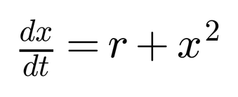
Here x represents the state of the system — think of it as a composite index of network health, where x=0 is normal operation. The parameter r represents the net stress on the system: the accumulation of traffic load, active intrusions, technical debt, staff fatigue, deferred maintenance, and the thousand small compromises that accrete in any large organisation like sediment in a riverbed.

When r is negative — when the system has margin — this equation has two equilibria, found by setting dx/dt=0:

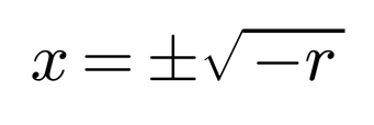
The negative root (x_=-√-r) is a stable equilibrium — the system’s normal operating state, the valley floor where the ball rests. Small perturbations (a traffic spike, a failed disk, a misconfigured rule) decay back to it. This is the behaviour we expect and the behaviour our dashboards report. The positive root (x₊=+√-r) is an unstable equilibrium — a repeller, the ridge line above the valley. On one side the ball rolls back to safety; on the other it rolls into catastrophe.

A point of precision, since the rest of this section depends on getting it right. This is a saddle-node bifurcation, but the name is borrowed from the higher-dimensional picture, where a saddle and a node collide. In our one-dimensional equation there is no saddle in the strict sense — both equilibria are simply fixed points, one stable and one unstable. Calling x₊ an “unstable repeller” is exact; calling it a “saddle point” would be a category error that a dynamicist would catch. The geometry is what matters: two fixed points, approaching each other.

Now consider what happens as stress increases — as r rises toward zero. The valley floor and the ridge line converge. And here is the crucial, terrifying insight: the system’s observable behaviour does not change during this process. Latency is normal. CPU load is manageable. Error rates are within tolerance. The dashboard remains a reassuring sea of green. The ball is still in the valley; it has not moved. But the valley has become shallower, the ridge lower. The resilience — the distance between where the system is and where it fails — is vanishing. We can quantify this precisely. The distance between the stable and unstable equilibria is:

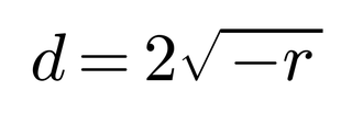
This quantity — the distance to bifurcation — is the true measure of the system’s remaining margin. And it shrinks continuously, silently, invisibly to any tool that monitors only the current state. At r=0 the two equilibria collide and annihilate. This is the bifurcation point. For r>0 no equilibrium exists; there is no stable state for the system to occupy. It is forced into rapid, discontinuous collapse — a free fall to a distant attractor, which in operational terms means catastrophic, system-wide failure. Not a degradation. Not a wobble. A cliff.

This geometry explains a pattern every network engineer has witnessed but linear monitoring cannot account for: the system that was “fine” five minutes ago and is now in total failure. The incident report will speak of a “sudden” outage, a “cascade” that “came from nowhere.” But the cascade did not come from nowhere. It came from the slow, invisible erosion of the distance to bifurcation. The system had been walking toward the cliff edge for weeks; the final step was unremarkable. It was the preceding steps that mattered, and no one was watching those. The monitors were tracking x — the position of the ball — when they should have been tracking r — the depth of the valley. Health monitoring measures where you are. Resilience monitoring measures how far you are from the cliff edge. The industry has invested billions in the former and barely begun to think about the latter.

A key implication for our digital twin is that it must be instrumented to estimate r, not just x. In practice this means tracking second-order indicators — the canaries that sing not of current failure but of approaching fragility: the rate at which recovery time is increasing after minor perturbations, the narrowing of operating margins between peak load and capacity, the accumulation of individually insignificant unresolved alerts that collectively signal a system under mounting strain.

There is an additional subtlety that offers a genuine lifeline. Near the bifurcation point a system exhibits critical slowing down: its recovery from small perturbations becomes measurably slower. A router that used to recover from a traffic spike in 200 milliseconds now takes 800. A service that used to self-heal in seconds now takes minutes. Nothing has “failed” — every component is within parameters — but the dynamic signature of impending collapse is present in the data, like the tremor before the earthquake. This is a detectable early-warning signal, and it has been validated across domains: in lakes approaching eutrophication, in financial markets approaching crashes, in climate systems approaching tipping points. Our Blue Agents can be trained to listen for the slowing heartbeat of a system approaching its bifurcation. It is, perhaps, the single most valuable contribution nonlinear dynamics can make to network resilience: a way to hear the cliff edge approaching, even when every dashboard says the ground is solid.

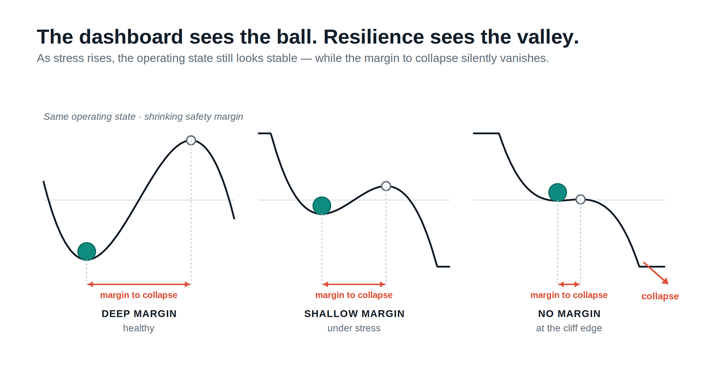
Figure 4. The dashboard sees the ball; resilience monitoring sees the valley. The current state can look stable while the basin silently becomes shallow.

3. Self-Organised Criticality: The Economics of the Sandpile

The bifurcation framework tells us what happens at the tipping point. But it leaves a deeper question unanswered: why do systems drift toward the tipping point in the first place? If the cliff edge is so dangerous, why do systems not stay safely in the middle of the valley?

The answer lies in Self-Organised Criticality (SOC), developed by Per Bak, Chao Tang, and Kurt Wiesenfeld in a landmark 1987 paper, and most famously illustrated by the sandpile model. Imagine dropping grains of sand, one at a time, onto a flat surface. A pile forms; as it grows, its slope steepens. For a while each grain simply adds to the pile. But as the slope approaches a critical angle, the system enters a different regime. Now the next grain might cause nothing — or it might trigger an avalanche of any size. The pile has organised itself, without external direction, into a critical state poised on the boundary between stability and collapse.

The key insight is the distribution of avalanche sizes, which follows a power law,

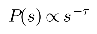
where s is the avalanche size and 𝜏 a scaling exponent typically between 1 and 2. This is not a bell curve. There is no “typical” avalanche. Small cascades are common; massive ones are rare but are an intrinsic statistical property of the system in its critical state. There is no “special” grain that causes the big avalanche — the same grain that yesterday caused a minor trickle causes today’s catastrophe. The difference is not in the trigger. It is in the state of the pile.

This is a philosophical point of immense practical importance. When we conduct root-cause analysis on a major outage, we instinctively look for a proportionate cause — a dramatic trigger worthy of the dramatic outcome. We look for the negligent engineer, the unpatched server, the sophisticated attacker. But SOC tells us the cause of a catastrophic cascade can be utterly mundane. The system was at criticality; any sufficiently unlucky perturbation would have triggered the collapse. The root cause is not the grain of sand. It is the slope of the pile. And the slope is shaped by something more powerful than any individual failure: economics.

Telecommunications networks are driven toward criticality by the relentless pressure to optimise. Every redundant link removed saves money. Every server consolidated reduces cost. Every buffer eliminated improves efficiency. Each optimisation is rational, defensible in a quarterly review, justifiable to a shareholder. But the cumulative effect is a system poised at criticality. We have, grain by grain, built the sandpile to its critical angle — rationally, efficiently, with the full approval of the finance department — and now we are surprised when avalanches occur.

This is not idle theory imported from physics. It has an established precedent in the closest cousin of our own infrastructure: the electrical power grid. In a body of work spanning two decades, Dobson, Carreras, Newman, and colleagues showed that cascading blackouts in real and modelled power systems exhibit the signatures of self-organised criticality — power-law distributions of blackout size, driven by exactly the tension we have described: load growing under economic pressure while upgrades lag, pushing the grid toward its critical point. Their OPA model treats the grid as a system that slowly self-organises toward criticality and then relaxes through cascading failures of unpredictable size. If the power grid — older, simpler, and more heavily regulated than a modern telecommunications network — sits at self-organised criticality, the prior probability that our infrastructure does too is high. We are not the first to build a sandpile and call it efficiency.

To visualise this, we can borrow Scott Page’s image of basins of attraction. Picture the network’s state as a ball rolling on a landscape of hills and valleys. A stable operating state is a valley — a basin. Its depth represents resilience: how large a shock the system can absorb without being pushed over the ridge. Its width represents robustness: how many different kinds of perturbation it can tolerate. Optimisation acts as a geological force that reshapes this landscape. By removing slack, redundancy, and buffers, we do not change the ball’s current position — the system appears healthy, settling quickly to the bottom. But we lower the ridges and narrow the valley. We create a landscape that is beautifully smooth and efficient, and so shallow that a perturbation which would once have been harmlessly absorbed now sends the ball careering into the next valley. We have optimised our way to fragility. The basin has become a saucer.

The digital twin lets us map this landscape computationally. By running thousands of simulations with varying perturbations — traffic spikes, component failures, attacks, configuration errors — we can estimate the depth and width of the basin under current conditions. If a perturbation equivalent to a routine Monday-morning traffic spike is enough to push the system over the ridge during a maintenance window, we have discovered that the basin has become critically shallow. We know the sandpile’s slope is at its critical angle, and the next grain is a matter of when, not if. This is, perhaps, the most important operational insight of the entire series: the system can be at criticality while every component is functioning normally and every metric is within tolerance. The danger lies not in the state of the system but in the shape of the landscape around it — invisible to any tool that only monitors the state.

4. Topology: Adversarial Percolation in Scale-Free Networks We now turn from dynamics to structure — from how systems collapse to where they are most vulnerable. For this we need percolation theory, drawn from statistical physics, which studies a question of deceptive simplicity: if we remove nodes from a network, at what point does it fragment into disconnected islands?

Imagine a regular grid of nodes connected to their neighbours. Remove a node at random; the network barely notices. Remove another, and another. For a long time it stays connected — there are always alternative paths. But at a specific fraction of removed nodes, the percolation threshold, the network undergoes a phase transition. The giant connected component shatters. Islands form. Communication ceases. The network has percolated — like water through a sieve, the connections have become too sparse to sustain continuity.

For a random network (an Erdős–Rényi graph), this threshold is relatively high; you must destroy a substantial fraction before fragmentation. Random networks are structurally democratic — no node is dramatically more important than any other — and this democracy confers resilience. But telecommunications networks are not random. As established by Barabási and Albert through preferential attachment, real-world networks — the internet, telecommunications infrastructure, social networks, the internal dependency graphs of enterprise IT — follow power-law degree distributions,

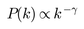
where k is a node’s number of connections and 𝛾 typically lies between 2 and 3. These are scale-free networks, and their structure is aristocratic — dominated by a few massively connected hubs and a long tail of sparsely connected peripheral nodes. The network is held together not by the collective strength of the many but by the structural importance of the few. It is less a fishing net (uniform, resilient, democratic) and more a spider’s web (beautiful, efficient, utterly dependent on its central radials).

Scale-free networks have a paradoxical property that encapsulates one of nature’s cruellest jokes. Under random failure — the daily attrition of hardware faults, software crashes, and human error — they are extraordinarily robust. Following Cohen and colleagues, the critical fraction of nodes that must be removed to fragment the network is:

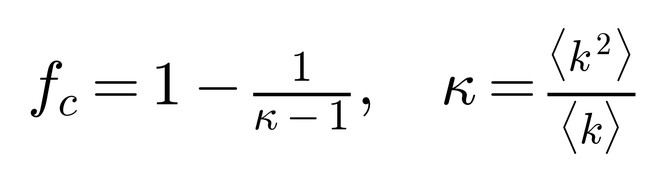
For scale-free networks with 𝛾 ≤ 3 , the second moment ⟨k²⟩ diverges (or, in finite networks, grows very large), driving k ➝ ∞ and fc➝ 1. You would have to destroy nearly the entire network to fragment it by random removal. This is why the internet “routes around damage,” why most hardware failures are invisible to end users. Against random perturbation the network is magnificently resilient.

But the joke has a punchline. Under targeted attack — the deliberate removal of the highest-degree nodes first, the strategy any intelligent adversary would pursue — the picture inverts with breathtaking completeness. Albert, Jeong, and Barabási demonstrated in a 2000 paper that removing even a small fraction of hubs causes the giant component to disintegrate; in simulations of real topologies, targeted removal of fewer than 5% of nodes can reduce the largest connected component by over 80%. The network that was nearly indestructible against accident is catastrophically fragile against intelligence. Resilience against random failure and resilience against targeted attack are not merely different quantities; in scale-free networks they are inversely related. The very structure that makes the network robust against the former makes it vulnerable to the latter. This is, mathematically, the worst possible security architecture: a system that shrugs off a thousand random failures and collapses under a single targeted strike.

A sophisticated adversary — our Red Agent — does not strike randomly. It performs reconnaissance, maps the topology, calculates betweenness centrality, and targets the nodes whose removal maximises fragmentation. The attacker’s optimisation problem is the exact dual of the defender’s: the defender seeks to maximise the percolation threshold, the attacker to minimise it. It is a mathematical arms race, and the attacker has a structural advantage — it is easier to identify hubs (they are, by definition, visible) than to protect them.

For the digital twin, this means we must compute and continuously monitor graph centrality metrics across the live infrastructure — not just for routers and switches but for every node in the dependency graph: authentication servers, DNS resolvers, licence managers, database clusters, and the human teams that operate them. A team of three engineers who are the sole holders of institutional knowledge about a legacy system are, in network-theoretic terms, a hub; their simultaneous absence (illness, holiday, resignation) is a targeted removal. The simulation can ask: “if the Red Agent compromises this specific node, what fraction of the network becomes unreachable?” When the answer exceeds an acceptable threshold, that node must be hardened, replicated, or structurally isolated — regardless of its perceived importance in the asset register, and regardless of whether it has ever appeared on a risk matrix. The mathematics does not care about organisational hierarchies. It cares about topology.

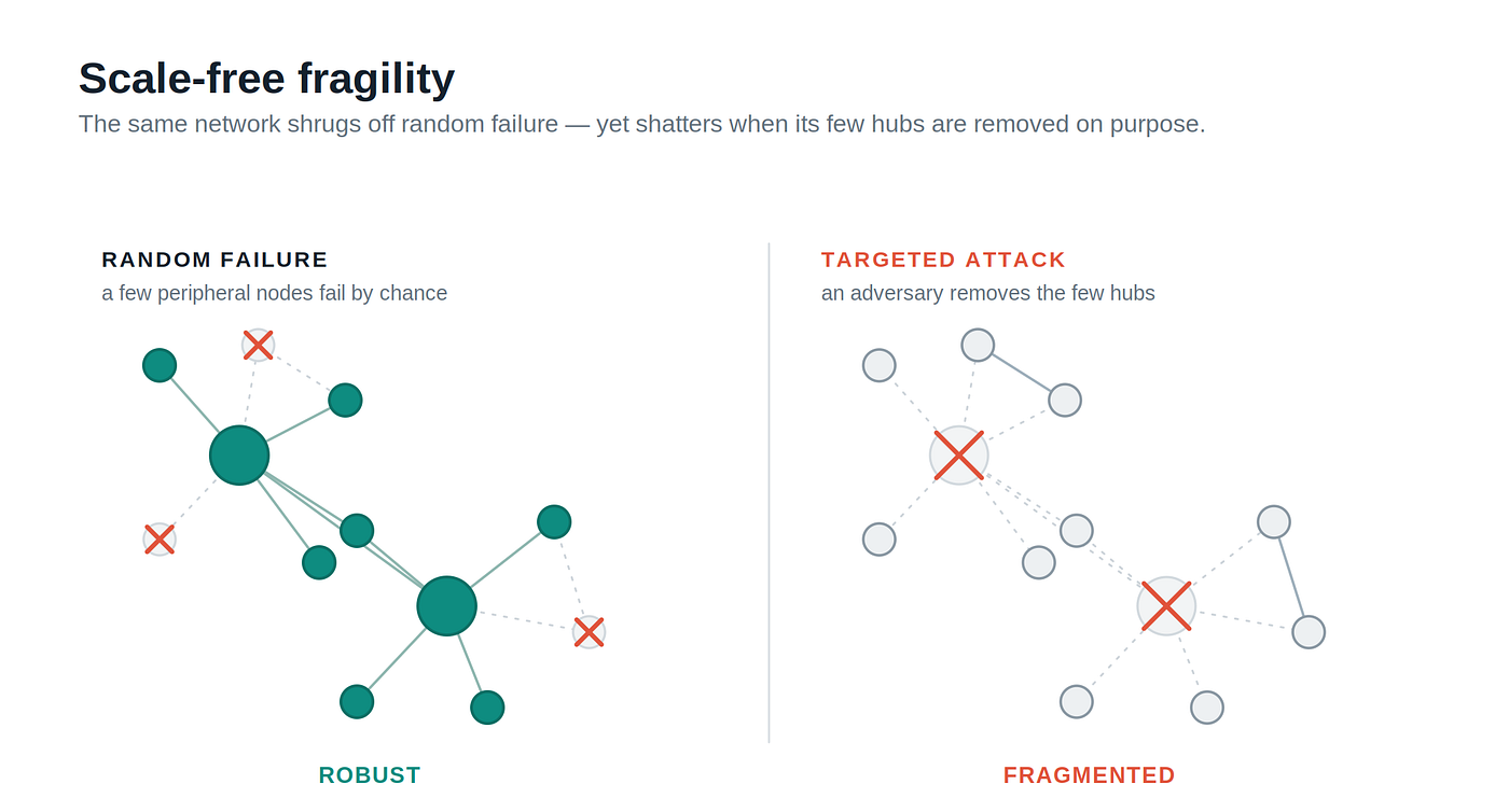
Figure 5. Scale-free fragility: a network can withstand random failures yet fragment rapidly under targeted hub removal.

A further implication involves what Duncan Watts called cascade conditions — the rules governing when a local failure becomes a global contagion. In Watts’s threshold model a node fails if more than a fraction of 𝜙 its neighbours have failed. A node of degree k is vulnerable — a single failed neighbour suffices to topple it — precisely when

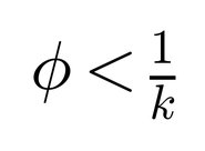
A note of care, because the literature is often quoted loosely here. This 𝜙 < 1/k is the condition for an individual node to be vulnerable, not the full condition for a global cascade. A system-wide cascade requires, in addition, that these vulnerable nodes form a connected cluster large enough to percolate — the vulnerable cluster must itself span the network. With that caveat, the result is genuinely counterintuitive and genuinely useful. High-degree hubs, while structurally critical, are the most resistant to cascade pressure — they require a large absolute number of failed neighbours to topple. Low-degree peripheral nodes are the most susceptible. A cascade therefore propagates through the periphery like a fire through dry brush, progressively surrounding the hubs until even they are overwhelmed. The collapse comes not from a frontal assault on the stronghold but from the encirclement of the countryside. The digital twin must model this dynamic — the slow encroachment, the tightening noose — not just the static topology.

5. The Epidemiology of Compromise: R₀ and the Vanishing Threshold Percolation tells us when a network fragments under node removal. But malware, a worm, a ransomware strain, or a lateral-movement campaign does not remove nodes — it infects them, and infected nodes infect others. This is not a question of structure but of spread over time, and the discipline that has spent a century mastering the mathematics of spread is epidemiology.

The mapping is almost embarrassingly direct. Replace “person” with “host,” “infection” with “compromise,” and “recovery” with “patched and re-imaged,” and the compartmental models that epidemiologists use to forecast measles and influenza describe the propagation of a worm through a network. In the SIS model (Susceptible–Infected–Susceptible), a host can be compromised, cleaned, and compromised again — which is exactly the life of a vulnerable server in an environment where the underlying flaw is never fully eliminated. In the SIR model (Susceptible–Infected–Recovered), once a host is properly patched it becomes immune — the right model for a one-off campaign against a now-closed vulnerability.

The single most important quantity epidemiology gives us is the basic reproduction number, R₀: the expected number of secondary infections produced by one infected individual in a fully susceptible population. The intuition is simple and powerful. If R₀ > 1, each infection more than replaces itself and the outbreak grows. If R₀ < 1, the chain of transmission dies out. The entire art of public health is driving R₀ below one (just as we saw in the global COVID-19 pandemic) — through vaccination (reducing the susceptible pool), through quarantine (reducing contact), through faster recovery (reducing the infectious period). Every one of those levers has a direct analogue in network defence: patching is vaccination, segmentation is quarantine, and rapid detection-and-reimage is a shortened infectious period. The value of R₀ is that it converts the vague question “will this spread?” into a single number that defenders can compute and, crucially, target. It is a more rigorous handle on contagion than the entropy fever chart of the next section — where entropy measures our uncertainty about the system, R₀ measures the system’s intrinsic tendency to spread, and the two answer different questions.

Now for the result that should make any CNI defender sit up. In a well-mixed population the epidemic threshold is clean: the infection spreads only if the transmission rate exceeds a critical value. But Pastor-Satorras and Vespignani showed, in a celebrated result, that on a scale-free network the epidemic threshold can vanish entirely. The threshold is governed by the same ratio that governed percolation,

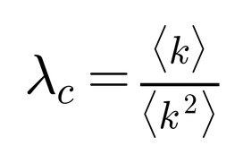
and for scale-free networks with 𝛾 ≤ 3 the divergence of ⟨k²⟩ drives 𝜆c ➝ 0. In plain terms: on a scale-free network, even a weakly contagious pathogen can spread to a finite fraction of the network. There is no safe level of contagiousness. A worm that would fizzle out on a regular grid can become endemic on the internet’s topology, because the hubs act as superspreaders — infected early, connected to thousands, broadcasting the contagion across the network before the defenders have finished writing the first incident ticket.

This is the dynamic counterpart of the percolation result, and it strengthens the same uncomfortable conclusion from a different direction. The scale-free structure that makes our networks robust against random hardware failure makes them not only fragile against targeted attack but hospitable to contagion. The two results rhyme because they are governed by the same moment of the degree distribution, ⟨k²⟩ — the mathematical fingerprint of the hubs.

The operational payoff is concrete and, pleasingly, optimistic. The same theory that delivers the bad news delivers the remedy: targeted immunisation. Because the hubs drive the epidemic, vaccinating them — hardening, monitoring, and segmenting the highest-degree nodes — collapses the spread far more efficiently than uniform defence, restoring a finite threshold to a network that otherwise has none. This is the epidemiological twin of the Pareto-tiering argument of Part 1, and it converts that argument from an appeal to the 80/20 rule into a theorem about epidemic thresholds. The digital twin can estimate the effective R₀ of a given threat against the current topology, identify the superspreader nodes, and quantify exactly how much a targeted-immunisation policy reduces it. We can ask: “does segmenting these twelve hubs pull R₀ below one for this strain of ransomware?” — and answer it before the strain arrives, rather than after.

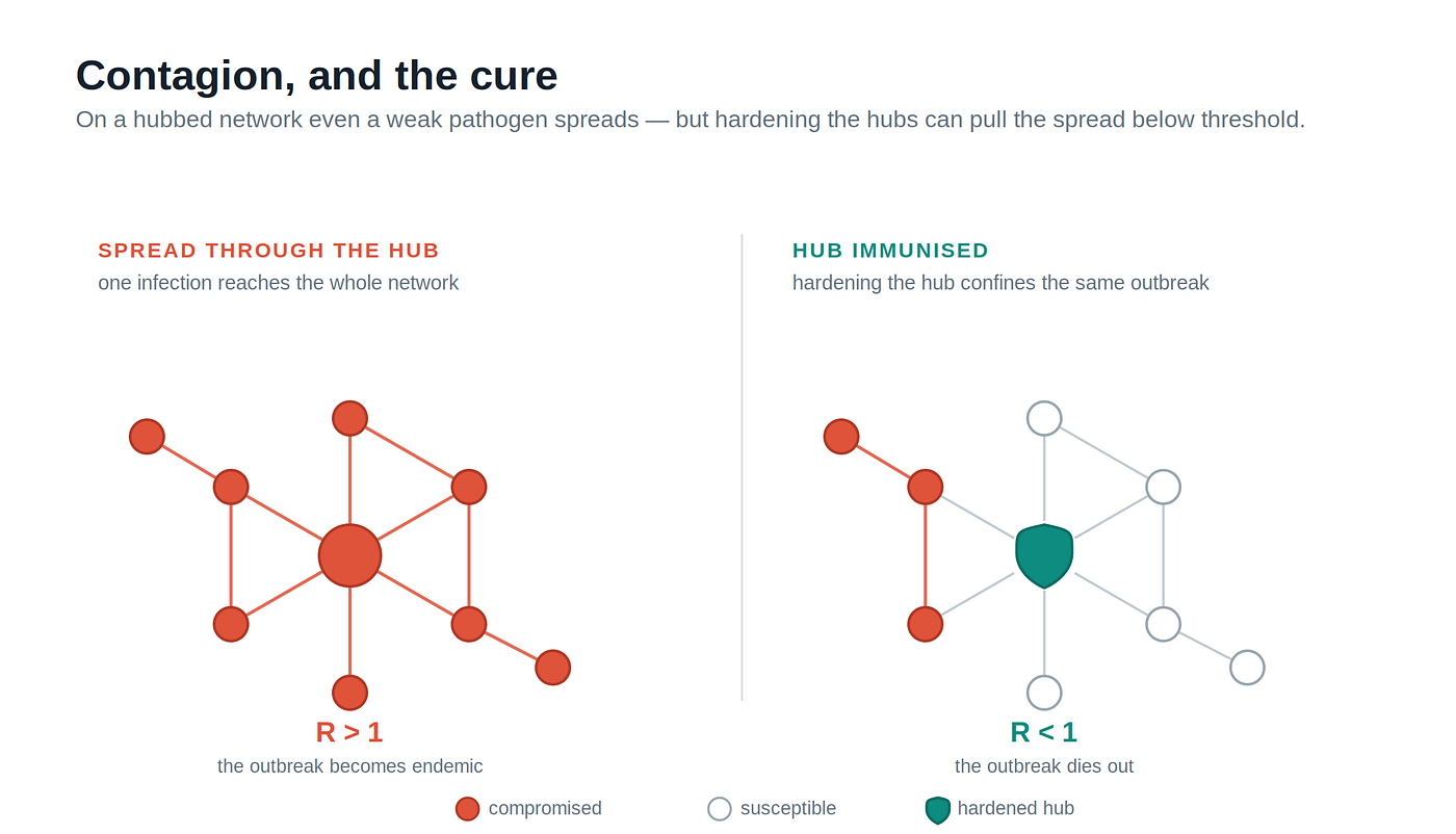
Figure 6. Contagion and targeted immunisation: hardening the hubs can change the reproduction dynamics of compromise.

6. Information Theory: The Fever Chart of Cyber War We have addressed the geometry of collapse, the topology of fragility, and the epidemiology of spread. We now need a thermometer — a metric for the state of health of the network as it undergoes adversarial pressure. For this we turn to one of the most profound intellectual achievements of the twentieth century: Claude Shannon’s information theory.

In a well-ordered, secure network the distribution of system states is concentrated and predictable. We know what software is running, who has access, what traffic patterns to expect. This order — this predictability — can be characterised using Shannon entropy,

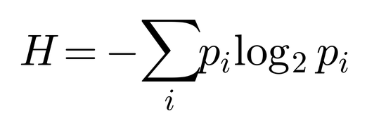
where the sum is over the possible states i of the system and 𝑝ᵢ is the probability of each. A fully determined system (one state with probability 1) has H=0; a system in which all states are equally likely has maximum entropy. Entropy, in Shannon’s formulation, is not disorder in the colloquial sense. It is uncertainty. It measures how much we don’t know about the state of the system.

A cyber attack is, in information-theoretic terms, an entropy injection. Every action the attacker takes increases the number of plausible system states, widening the cloud of uncertainty the defenders must contend with. Are these files intact or modified? Has this account been compromised or is it legitimate? Is this routing table correct or has it been poisoned? Each successful attacker action smears the distribution, increasing H. The attacker is injecting doubt — and doubt, quantified as entropy, is the true weapon of cyber warfare. The defence — the Security Operations Centre — is an entropy reduction process: each confirmed investigation (“this server is clean”) and each successful remediation (“this system has been re-imaged from a verified backup”) collapses uncertainty and reduces H. The SOC is fighting uncertainty with knowledge.

We can formalise the contest as a rate equation — a fever chart for the battle. Let Ṡattack be the rate at which Red Agents inject entropy and Ṡdefend the rate at which Blue Agents export it through investigation and remediation. The net entropy change is

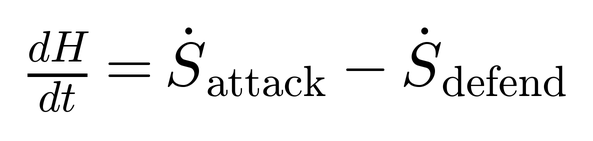
The sign determines who is winning. If dH/dt < 0, the defenders are resolving uncertainty faster than the attacker creates it; the fog is lifting. If dH/dt > 0, the attackers are winning; compromised systems accumulate, unverified alerts pile up, and the SOC’s mental model diverges further from reality. If this persists, the system approaches maximum entropy — a state where operators cannot distinguish compromised components from clean ones — and the only viable strategy is often a complete rebuild: the “nuke it from orbit” scenario, the most expensive and humiliating outcome possible. If dH/dt=0, the battle is a stalemate — the “persistent compromise” that endures for months, draining resources and corroding trust.

This framing gives the simulation a quantitative objective function. We can measure the trajectory of H over time in each run, identify the conditions under which dH/dt flips from negative to positive, and test whether a specific capability — a new detection tool, an extra analyst on shift, automated containment — changes the sign under a given attack scenario. Security investment becomes a measurable question: does this expenditure reduce the rate of entropy accumulation under our worst-case scenarios?

A note of intellectual honesty, because precision matters and overreach undermines credibility. This is Shannon entropy applied by analogy to network states, not a direct application of thermodynamic entropy governed by the second law. The SOC is not literally Maxwell’s Demon; the network is not a thermodynamic system in equilibrium; Landauer’s principle does not apply to firewall rules. And there is a second honesty owed here that the original framing glossed: of all the tools in this essay, entropy is the least directly operationalisable. The bifurcation distance d=2√-r, the percolation threshold fc, and the reproduction number R₀ can each, in principle, be estimated from measurable quantities. The entropy fever chart, by contrast, requires us to define a state space and a probability distribution over it that no production network exposes directly — so in practice H is a constructed proxy (over alert states, asset-integrity states, identity-confidence states) rather than a measured quantity. Treated as an organising heuristic that captures what practitioners feel in their bones — that attacks create disorder and defences restore order, and the balance of rates determines the outcome — it is illuminating. Treated as a precise instrument, it would be overclaiming. We use Shannon’s mathematics because uncertainty is the currency of cyber warfare and his is the right language for reasoning about it, not because the network is a thermodynamic engine.

7. Synchronisation: The Thundering Herd and the Rhythm of Vulnerability We must also consider a failure mode that arises not from individual weakness or structural fragility but from collective dynamics — synchronisation. It is, in its way, the most elegant and the most treacherous, because it emerges from components doing exactly what they were designed to do, just doing it at the wrong time.

The classic example is the thundering herd. After a brief network outage, thousands or millions of devices attempt to reconnect simultaneously. Each device follows its recovery protocol correctly. But because the outage affected all of them at the same instant, their recovery cycles are now aligned, and the resulting demand spike can exceed the network’s capacity by orders of magnitude — causing the very outage the devices are recovering from. The system is trapped in a loop: outage → synchronised recovery → overload → outage. The cure causes the disease that necessitates the cure. It is Sisyphus, implemented in silicon.

It is worth being precise about the mechanism, because the original telling of this story reached for the wrong model. There are two distinct routes to synchronisation, and they are not the same. The thundering herd is common-mode synchronisation: the devices align not because they are coupled to one another but because they were all subjected to the same shock at the same moment and share the same recovery timer. This is a correlated initial condition, best modelled as a population of pulse-coupled oscillators kicked simultaneously, and its remedy is to break the correlation.

The second route is the one the Kuramoto model properly describes: spontaneous synchronisation that emerges from coupling between oscillators with different natural frequencies. For N coupled oscillators with phases Øⱼ, the degree of synchronisation is captured by an order parameter,

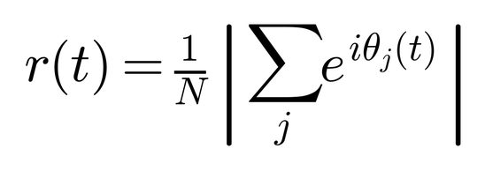
When r≈0 the oscillators are desynchronised, their phases spread out and their aggregate demand smooth. When r➝1 they are locked, all peaking together, creating spikes that shatter capacity limits. Above a **critical coupling strength **Kc, synchronisation emerges spontaneously — a phase transition in the collective behaviour of the network’s components. This is the right model when the components genuinely influence one another’s timing: backup jobs that trigger off a shared signal, autoscaling groups that react to the same metric, retry logic that couples through a common queue. The thundering herd and the Kuramoto cascade can look identical on a demand graph, but they have different causes, and conflating them leads to the wrong fix.

The good news is that the fix is the same in both cases, even though the diagnosis differs: deliberate jitter — randomising the timing of periodic operations — breaks common-mode alignment and, in the coupled case, pushes the system below Kc. The digital twin earns its keep here in two ways. Defensively, it can test whether the operational rhythms of the infrastructure — patch cycles, polling intervals, backup schedules, health checks, certificate renewals — create hidden synchronisation an attacker could exploit. If every router in a region backs up at midnight, every firewall refreshes its rules at midnight, and the monitoring system runs its heaviest analysis at midnight, then midnight is a window of simultaneous vulnerability as predictable as a heartbeat. A Red Agent that learns these rhythms can strike between the beats. Operationally, the simulation can quantify exactly how much jitter is needed — enough to desynchronise the peaks, not so much that the operations themselves become unreliable. It is a delicate calibration, and the twin is the only safe place to find the balance.

This connects to the edge of chaos — the notion, from Christopher Langton’s work on cellular automata, that complex adaptive systems tend to operate near the boundary between ordered and chaotic regimes. In the ordered regime a system is stable but rigid; in the chaotic regime it is flexible but uncontrollable; at the boundary it achieves maximum adaptive capacity. Whether telecommunications networks literally occupy this regime is an empirical question, not an axiom — and one the twin can investigate by measuring the system’s Lyapunov exponents, the rates at which nearby trajectories in state space diverge. Negative exponents mean perturbations decay (the ordered regime); positive exponents mean they grow exponentially (chaos); exponents near zero mean the critical boundary. A positive largest Lyapunov exponent is the mathematical signature of chaos: prediction becomes exponentially harder with time, the system’s future exquisitely sensitive to its present. If our network operates in the chaotic regime we need to know it, because long-term prediction becomes impossible and strategy must shift from prediction to preparedness. Moving this from a suggestive metaphor to a tested, quantified hypothesis is one of the contributions the digital twin can make.

8. The Mathematics of Overload: Queues, Utilisation, and the Other Cliff There is a second cliff in our infrastructure, quite different in mechanism from the bifurcation but uncannily similar in operational signature, and it lives inside one of the most practical branches of mathematics: queueing theory, the discipline that operations researchers built to understand call centres, motorways, and any system where work arrives and waits to be served.

Every component that processes work — a router forwarding packets, a firewall inspecting connections, a SOC analyst triaging alerts — is a server in front of a queue. Two quantities govern its behaviour: the rate at which work arrives, 𝜆, and the rate at which it can be served, 𝜇. Their ratio, the utilisation 𝜌=𝜆/𝜇, is the fraction of capacity in use, and it is the most treacherous number in the system. The relationship that should be tattooed on every capacity planner’s forearm is the behaviour of the mean waiting time in a simple queue,

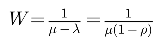
Read that denominator carefully. As utilisation 𝜌 approaches 1 — as arrivals approach capacity — the waiting time does not rise gently. It diverges to infinity. At 80% utilisation a system is comfortable. At 95% it is straining. At 99% the queue, and the latency, blow up. This is the other cliff: not the disappearance of an equilibrium, as in the bifurcation, but the explosion of delay as a system is pushed toward full utilisation. The two mechanisms are mathematically distinct — one is a saddle-node bifurcation in a dynamical system, the other a singularity in a queue — yet to an operator they present the same way: a system that was “fine” at 90% and unusable at 98%, with the last few percent of load triggering a collapse out of all proportion to the increase that caused it. Recognising which cliff you are standing on matters, because the remedies differ: the bifurcation calls for restoring margin to the dynamics, the queue for restoring headroom in capacity.

The companion result is Little’s Law, as close to a universal truth as queueing theory possesses:

L=𝜆𝘞

the average number of items in a system equals the arrival rate times the average time each spends there. Its beauty is its generality — it holds regardless of the distribution of arrivals or service times — and its reach into our problem is immediate. Consider the SOC. If alerts arrive at 𝜆 per hour and analysts can meaningfully process them at 𝜇 per hour, then as 𝜌 ➝ 1 the backlog L explodes and the time an alert waits before investigation diverges. Alert fatigue is not a psychological failing; it is a queueing singularity. The well-documented reality that a SOC receiving 500 alerts per shift can investigate only 40 is precisely the statement that 𝜌 ⨠ 1 for that queue, that the backlog grows without bound, and that the effective detection probability for any given true positive collapses as it sinks down an ever-lengthening queue. The attacker understands this implicitly: every action that raises the alert arrival rate — noise, decoys, a flood of low-severity events — pushes the defender’s queue toward its singularity, and a defender at 𝜌 > 1 is, in a rigorous sense, blind.

There is a final subtlety that queueing theory shares with the bifurcation story: metastability. A queue operating near capacity can sit in a deceptively stable state for a long time, then tip into a congested state from which it does not spontaneously recover, because the congestion itself degrades service (retries, timeouts, retransmissions) and pushes 𝜌 higher still — a positive feedback loop that locks the system in collapse. This is the queueing analogue of the auto-immune cascade, and it points directly at the next tool. For the digital twin, queueing theory supplies something the other instruments do not: a rigorous, quantitative account of capacity margin across every processing element in the network, human and machine alike, and a way to ask “how much spare headroom does this server, this link, this analyst team have before the latency cliff?” — and to discover where an adversary, or merely a bad Tuesday, could push the system over it.

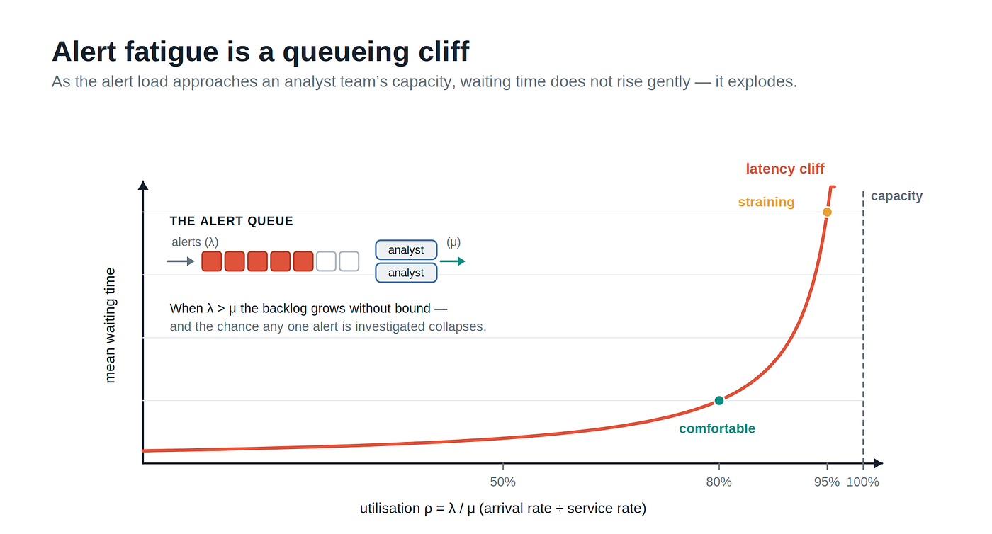
Figure 7. Alert fatigue as a queueing cliff: once arrivals approach service capacity, delay and backlog become nonlinear.

9. Feedback and Stability: When the Cure Oscillates We end the toolkit where Part 1 promised we would: with the mathematics that turns the “auto-immune response” from a vivid metaphor into a quantity an engineer can tune. The discipline is control theory, the century-old science of feedback that keeps aircraft level, reactors stable, and thermostats honest — and its central concern, stability, is exactly the concern Leveson’s STAMP raised when it reframed accidents as failures of control.

A control loop has three essential ingredients: it senses a deviation, it decides on a correction, and it acts. An automated defence is precisely such a loop. It senses an intrusion, decides on a containment action, and acts by isolating a subnet. The promise of feedback is stabilisation — pulling the system back toward safety. But control theory’s hardest-won lesson is that feedback can destabilise just as easily as it stabilises, and it tells us, with precision, when. Two quantities decide the matter: the gain of the loop (how aggressively it responds to a deviation) and the delay, or phase lag, between sensing and acting. When a loop combines high gain with significant delay, its corrections arrive out of phase with the problem — the controller is fighting yesterday’s fire with today’s water — and instead of damping the disturbance it amplifies it. The system begins to oscillate, and if the loop gain at the oscillation frequency exceeds unity, the oscillation grows until something saturates or breaks. This is not a metaphor; it is the Nyquist stability criterion, and it is why a poorly tuned cruise control surges, why a public-address system howls, and — we now argue — why an automated containment system can tear a network apart.

The auto-immune cascade we will dissect in Part 3 is, in this light, a textbook closed-loop instability. The defensive controller responds to an intrusion (high gain: it isolates an entire subnet) on the basis of information that is already stale (delay: the OODA loop from detection to action takes minutes, during which the situation moves). Its action shifts load onto adjacent subnets, pushing them toward their own limits — and when they fail, the controller responds again, more aggressively, on information that is staler still. Each correction arrives out of phase with the threat and adds energy to the disturbance rather than removing it. In Leveson’s vocabulary this is an unsafe control action; in control theory’s it is a loop with too much gain and too much delay, operating beyond its stability margin. The two descriptions are the same phenomenon seen through different lenses, and together they tell us exactly what to measure: the gain of every automated response, the delay in every feedback path, and the stability margin — how much we could increase the gain, or the delay, before the loop tips into oscillation.

The remedies are not vague exhortations to “be careful.” They are the standard toolkit of control engineering, and they map one-to-one onto the security mitigations the original series proposed by intuition. Reduce the gain: cap the rate at which automated isolation can occur, so the system shifts load gradually rather than in destabilising lurches. Add damping: introduce the randomised delays — the jitter of the previous section — that prevent defensive actions from resonating with the attack. Add hysteresis: require a containment action to clear a higher threshold to engage than to disengage, so the controller does not chatter on the boundary. Shorten the delay: invest in faster, higher-fidelity detection so the loop acts on fresh information and its corrections arrive in phase. Each of these has a precise effect on the stability margin, and each can be implemented in the simulation, tested against adaptive Red Agents, and tuned. The digital twin becomes a stability-analysis bench for the organisation’s defensive control loops — the only safe place to discover that your immune system, like an over-eager autopilot, is allergic to itself.

10. Conclusion: The Cartography of Catastrophe We have assembled a toolkit — a set of lenses through which to view the dynamics of failure in complex telecommunications infrastructure, each borrowed from a discipline that learned it the hard way:

Bifurcation theory reveals the cliff edges that do not appear on dashboards — the silent erosion of resilience captured by d=2√-r, and the lifeline of critical slowing down. Self-organised criticality explains why those cliff edges sit terrifyingly close, driven there by the economics of optimisation — a phenomenon already documented in the power grid. Percolation theory maps the Achilles’ heels of the network’s topology through fc=1–1/(𝜅-1), and the epidemiology of compromise turns the spread across that topology into the reproduction number R₀, with the chilling result that scale-free networks can have no epidemic threshold at all — and the consoling corollary that immunising the hubs restores one. Shannon entropy provides a fever chart for the information war via dH/dt=Ṡattack-Ṡdefend, honestly held as a heuristic rather than an instrument. Queueing theory exposes the second cliff, the latency singularity as utilisation 𝜌 ➝ 1, and reframes alert fatigue as a queueing phenomenon. And control theory turns the auto-immune response into a stability margin, telling us precisely when feedback heals and when it howls.

Each of these tools, applied in isolation to a simplified model, yields analytical insight — clean, elegant, and insufficient. The telecommunications CNI is not a simplified model. It is a system in which bifurcation dynamics interact with percolation topology, in which contagion alters the effective coupling between oscillators, in which queue congestion feeds control-loop instability, and in which the adaptive behaviour of human operators feeds back into every layer. The interactions create a phase space of such dimensionality that closed-form analytical solutions are unattainable. We are in the realm the mathematicians, with their gift for understated despair, call “analytically intractable.”

Stephen Wolfram captures this with the concept of computational irreducibility: for many complex systems there is no shortcut to predicting their behaviour. You cannot derive the future from an equation; you must run the computation. The future is not a formula to be solved but a programme to be executed.

We should be precise about what this means for our proposal, because intellectual honesty demands it. If the system is truly computationally irreducible in Wolfram’s strict sense, then no simulation can predict faster than the real system evolves — the twin would need to run at least as long as reality to produce accurate forecasts. We do not claim to have solved this. We claim something more modest and more useful. Our digital twin does not predict the future; it explores the distribution of possible futures. By running many simulations across a range of initial conditions, parameter uncertainties, and adversarial strategies, we map the statistical landscape of risk — which regions of parameter space lead to catastrophe and which do not. We cannot predict which grain of sand will trigger the avalanche, but we can measure the slope of the pile and estimate the distribution of avalanche sizes. We cannot foretell the earthquake, but we can map the fault lines. We trade the impossible goal of exact prediction for the achievable goal of probabilistic risk characterisation — not a defeat, but a mature acknowledgement of the nature of the systems we have built, and immeasurably more useful than the false certainty of a risk matrix.

This is the computational imperative that drives Part 3: the architecture of the digital twin itself — the machine that brings these tools to life, the macroscope that reveals the hidden cartography of catastrophe. We move from the equations to the engine; from the physics of failure to the engineering of foresight.

*Part 3: The Digital Twin — Architecting the Simulation of the Unseen*

References and Further Reading

The following sources underpin the arguments of this series. Where a concept is attributed to a particular author in the text, the foundational work is listed here. The list is organised by theme rather than alphabetically, to function as a guide for the reader who wishes to pursue any thread in greater depth.

Risk, Measurement, and Decision Under Uncertainty

Hubbard, D. W. (2020). The Failure of Risk Management: Why It’s Broken and How to Fix It (2nd ed.). Wiley.

Hubbard, D. W. (2014). How to Measure Anything: Finding the Value of Intangibles in Business (3rd ed.). Wiley. [Calibration training; the Rule of Five.]

Kahneman, D. (2011). Thinking, Fast and Slow. Farrar, Straus and Giroux. [Systematic miscalibration of intuition about rare events.]

Systems Safety and Resilience Engineering

Perrow, C. (1999). Normal Accidents: Living with High-Risk Technologies (2nd ed.). Princeton University Press. [Interactive complexity and tight coupling.]

Leveson, N. G. (2011). Engineering a Safer World: Systems Thinking Applied to Safety. MIT Press. [STAMP — accidents as inadequate control.]

Leveson, N. G., & Thomas, J. P. (2018). STPA Handbook. [Method for enumerating unsafe control actions; freely available.]

Hollnagel, E. (2014). Safety-I and Safety-II: The Past and Future of Safety Management. Ashgate.

Hollnagel, E., Woods, D. D., & Leveson, N. (Eds.). (2006). Resilience Engineering: Concepts and Precepts. Ashgate.

Woods, D. D. (2015). “Four concepts for resilience and the implications for the future of resilience engineering.” Reliability Engineering & System Safety, 141, 5–9. [Graceful extensibility.]

Cook, R. I. (1998/2000). How Complex Systems Fail. Cognitive Technologies Laboratory, University of Chicago.

Nonlinear Dynamics, Chaos, and Self-Organised Criticality

Strogatz, S. H. (2015). Nonlinear Dynamics and Chaos (2nd ed.). Westview Press/CRC. [Bifurcations; the saddle-node; critical slowing down.]

Bak, P., Tang, C., & Wiesenfeld, K. (1987). “Self-organized criticality: An explanation of 1/f noise.” Physical Review Letters, 59(4), 381–384.

Bak, P. (1996). How Nature Works: The Science of Self-Organized Criticality. Copernicus.

Dobson, I., Carreras, B. A., Lynch, V. E., & Newman, D. E. (2007). “Complex systems analysis of series of blackouts: Cascading failure, critical points, and self-organization.” Chaos, 17(2), 026103. [The OPA model; SOC in power grids.]

Carreras, B. A., Newman, D. E., Dobson, I., & Poole, A. B. (2004). “Evidence for self-organized criticality in a time series of electric power system blackouts.” IEEE Transactions on Circuits and Systems I, 51(9), 1733–1740.

Langton, C. G. (1990). “Computation at the edge of chaos: Phase transitions and emergent computation.” Physica D, 42(1–3), 12–37.

Wolfram, S. (2002). A New Kind of Science. Wolfram Media. [Computational irreducibility.]

Network Science, Percolation, and Epidemic Spreading

Barabási, A.-L., & Albert, R. (1999). “Emergence of scaling in random networks.” Science, 286(5439), 509–512. [Scale-free networks; preferential attachment.]

Albert, R., Jeong, H., & Barabási, A.-L. (2000). “Error and attack tolerance of complex networks.” Nature, 406(6794), 378–382. [Robust-yet-fragile.]

Cohen, R., Erez, K., ben-Avraham, D., & Havlin, S. (2000). “Resilience of the Internet to random breakdowns.” Physical Review Letters, 85(21), 4626–4628; and (2001) “Breakdown of the Internet under intentional attack.” Physical Review Letters, 86(16), 3682–3685.

Watts, D. J. (2002). “A simple model of global cascades on random networks.” PNAS, 99(9), 5766–5771. [Threshold cascades; node vulnerability and the vulnerable cluster.]

Pastor-Satorras, R., & Vespignani, A. (2001). “Epidemic spreading in scale-free networks.” Physical Review Letters, 86(14), 3200–3203. [Vanishing epidemic threshold.]

Pastor-Satorras, R., Castellano, C., Van Mieghem, P., & Vespignani, A. (2015). “Epidemic processes in complex networks.” Reviews of Modern Physics, 87(3), 925–979. [Comprehensive review; targeted immunisation.]

Information Theory, Synchronisation, and Control

Shannon, C. E. (1948). “A mathematical theory of communication.” Bell System Technical Journal, 27, 379–423 and 623–656.

Strogatz, S. H. (2000). “From Kuramoto to Crawford: Exploring the onset of synchronization in populations of coupled oscillators.” Physica D, 143(1–4), 1–20.

Åström, K. J., & Murray, R. M. (2008). Feedback Systems: An Introduction for Scientists and Engineers. Princeton University Press. [Gain, delay, phase margin; the Nyquist criterion; stability margins.]

Queueing Theory

Kleinrock, L. (1975). Queueing Systems, Volume 1: Theory. Wiley. [M/M/1; utilisation and the latency singularity.]

Little, J. D. C. (1961). “A proof for the queuing formula: L = λW.” Operations Research, 9(3), 383–387.

Extreme Value Theory

Coles, S. (2001). An Introduction to Statistical Modeling of Extreme Values. Springer. [GEV, GPD, Peaks-Over-Threshold.]

Embrechts, P., Klüppelberg, C., & Mikosch, T. (1997). Modelling Extremal Events for Insurance and Finance. Springer. [Fisher–Tippett–Gnedenko; Pickands–Balkema–de Haan; the Hill estimator.]

Game Theory, Multi-Agent Learning, and Evolutionary Computation

Tambe, M. (2011). Security and Game Theory: Algorithms, Deployed Systems, Lessons Learned. Cambridge University Press. [Stackelberg security games in the field.]

Silver, D., et al. (2017). “Mastering the game of Go without human knowledge.” Nature, 550(7676), 354–359. [Self-play; co-evolution to superhuman skill.]

Holland, J. H. (1992). Adaptation in Natural and Artificial Systems. MIT Press.

Goldberg, D. E. (1989). Genetic Algorithms in Search, Optimization, and Machine Learning. Addison-Wesley.

Causal Inference

Pearl, J. (2009). Causality: Models, Reasoning, and Inference (2nd ed.). Cambridge University Press. [The do-operator; the ladder of causation.]

Pearl, J., & Mackenzie, D. (2018). The Book of Why: The New Science of Cause and Effect. Basic Books.

Ergodicity Economics

Peters, O. (2019). “The ergodicity problem in economics.” Nature Physics, 15, 1216–1221.

Peters, O., & Gell-Mann, M. (2016). “Evaluating gambles using dynamics.” Chaos, 26(2), 023103. [Ensemble average versus time average; ruin.]

Many-Model Thinking, Decision Cycles, and Adoption

Page, S. E. (2018). The Model Thinker: What You Need to Know to Make Data Work for You. Basic Books.

Page, S. E. (2007). The Difference. Princeton University Press. [The Diversity Prediction Theorem — exact for aggregating numerical predictions under squared-error loss.]

Osinga, F. P. B. (2007). Science, Strategy and War: The Strategic Theory of John Boyd. Routledge. [The OODA loop.]

Moore, G. A. (2014). Crossing the Chasm (3rd ed.). HarperBusiness.

Korzybski, A. (1933). Science and Sanity. [The map is not the territory.]

Agentic AI and Simulation Methods

Yao, S., et al. (2023). “ReAct: Synergizing Reasoning and Acting in Language Models.” International Conference on Learning Representations (ICLR).

Wu, Q., et al. (2023). “AutoGen: Enabling Next-Gen LLM Applications via Multi-Agent Conversation.” Microsoft Research.

MITRE. ATT&CK Framework (attack.mitre.org) and CALDERA (caldera.mitre.org); Red Canary, Atomic Red Team. [Adversary emulation and breach-and-attack simulation — established prior art.]

Metropolis, N., & Ulam, S. (1949). “The Monte Carlo method.” Journal of the American Statistical Association, 44(247), 335–341.

UK Regulation and Standards

Telecommunications (Security) Act 2021. UK Public General Acts. [Statutory security duties; Ofcom enforcement; penalties up to 10% of relevant turnover.]

The Electronic Communications (Security Measures) Regulations 2022 (SI 2022/933); Department for Science, Innovation and Technology, Telecommunications Security Code of Practice (2022); Department for Science, Innovation and Technology, Draft Revised Telecommunications Security Code of Practice 2026, published 3 June 2026, https://www.gov.uk/government/publications/draft-revised-telecommunications-security-code-of-practice-2026.

Cyber Security and Resilience (Network and Information Systems) Bill (2024–26 session; carried over and reintroduced at Report stage in the 2026–27 session; current Bill documents listed by UK Parliament in June 2026), https://bills.parliament.uk/bills/4035.

The Network and Information Systems Regulations 2018 (SI 2018/506). [The framework the CS&R Bill modernises.]

National Cyber Security Centre. (2025). Cyber Assessment Framework (CAF), Version 4.0 (released August 2025), and NCSC CAF changelog noting v4.0 release on 4 August 2025, https://www.ncsc.gov.uk/collection/cyber-assessment-framework/changelog.