PCB Card Comparison for Finding Defects (It Includes Python Image Comparison Methods)
This paper was written to compare two PCB samples and identify differences using image processing. This was the initial goal of the…
PCB Card Comparison for Finding Defects (It Includes Python Image Comparison Methods)
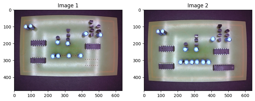
This paper was written to compare two PCB samples and identify differences using image processing. This was the initial goal of the research, but along the way, it became necessary to understand how to compare two images, which methods are suitable for this project, and how these methods work.
There are several methods for comparing two images in Python. Some return a numerical value, while others produce a difference image. This paper may not include all of them, but you will learn about many of them.
Method 1: Histogram Comparison
Histogram comparison is a more primitive way of comparing two images. In this method, you compare the color distribution of the images. For example, if you compare a red tomato and a green apple, the similarity ratio will be low and close to 0%. This means they aren’t similar. But if you compare a red tomato with a red apple, the similarity ratio will be high and close to 100%. This means they are similar. However, we know that tomatoes and red apples aren’t actually similar. The histogram method compares two images using color density. It is a basic and rapid method.

Similarity Ratio: 99.12%
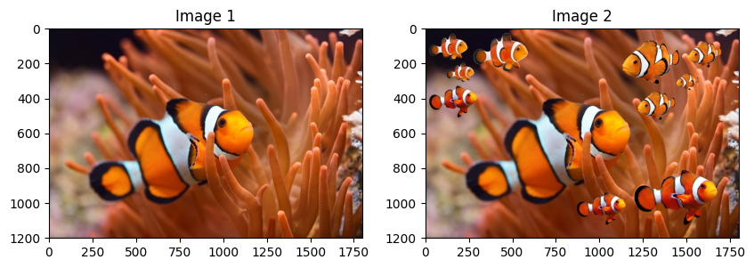
Similarity Ratio: 98.85%
Similarity Ratio: 89.62%
Method 2: Template Matching
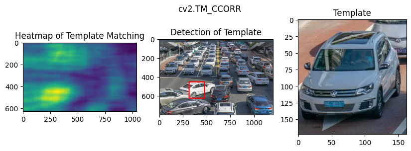
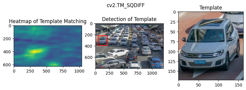
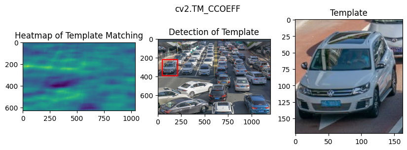
Template matching is a comparison method for finding a pattern or an object. This method has some limitations. When using template matching, you need to have a target image within the reference image. If the image is large, performance will be low due to the extensive calculations and potential mismatches.
Method 3: Feature Matching
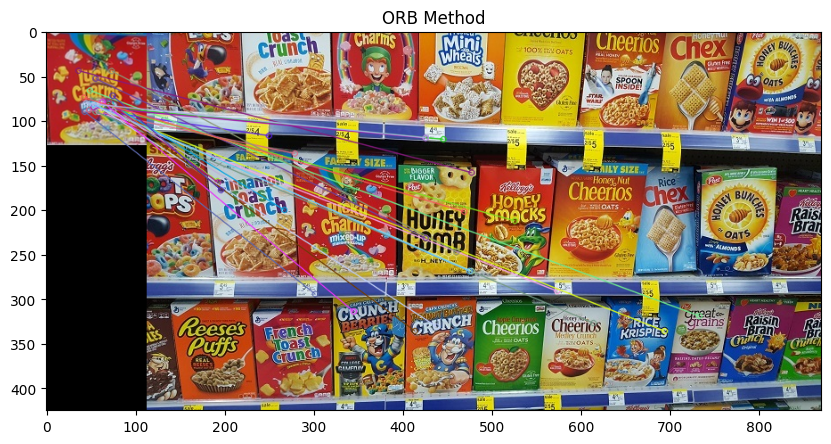
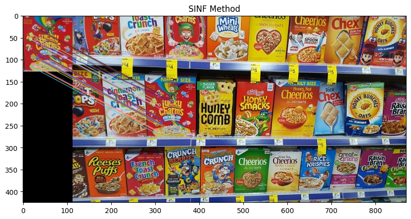
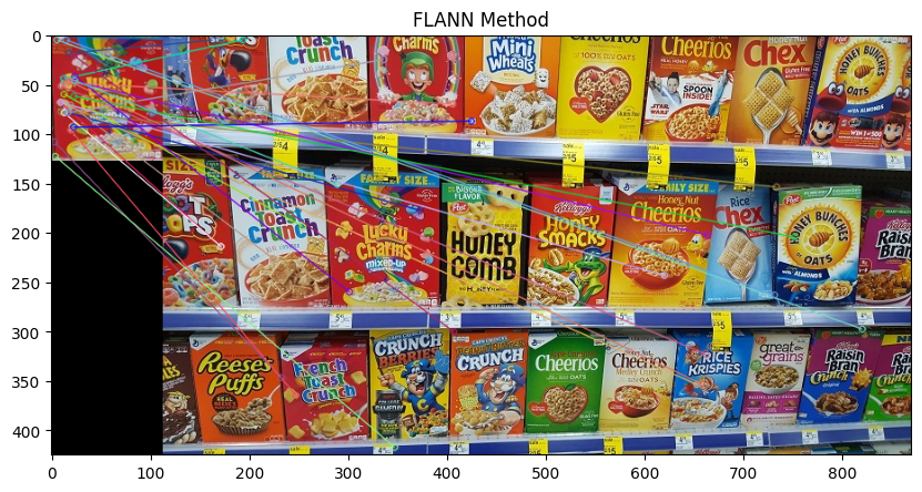
Feature matching is another way to match images. This method finds key points, defines descriptors for these points, and compares them to find corresponding points in another image. This method can handle images of different scales, sizes, or skewed orientations. There are more than three ways to perform feature matching. In this paper, only three of them are shown.
Method 4: Structural Similarity Index Measure (SSIM)
SSIM is a method for finding similarity between two images. This method is different from simple pixel-by-pixel methods. It considers luminance, contrast, and structure when making comparisons, which leads to a more accurate assessment of image similarity. The downside of this method is that it is more effective for images of the same scale. For complex images, it may not perform well.
SSIM returns a value between -1 and 1. A value of 1 indicates that the images are very similar, while a value of -1 indicates that the images are very different.
Similarity Score: 89.462%
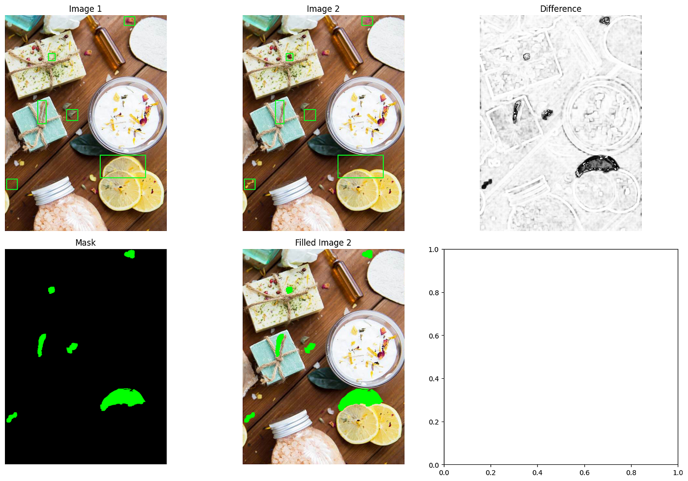
Similarity Score: 91.989%
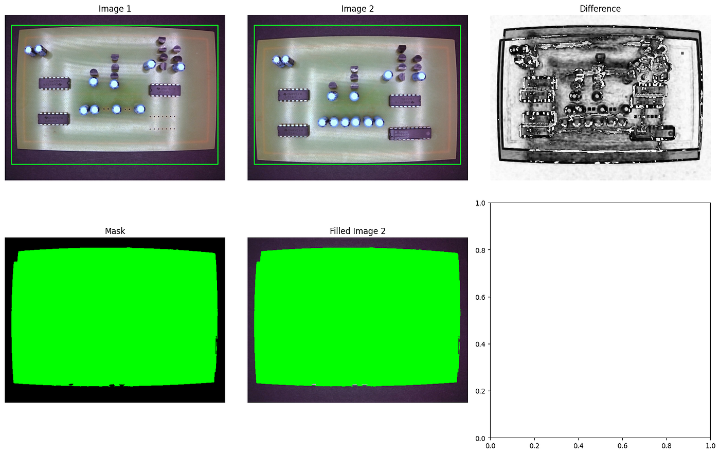
Similarity Score: 91.989%
Method 5: Absolute Difference
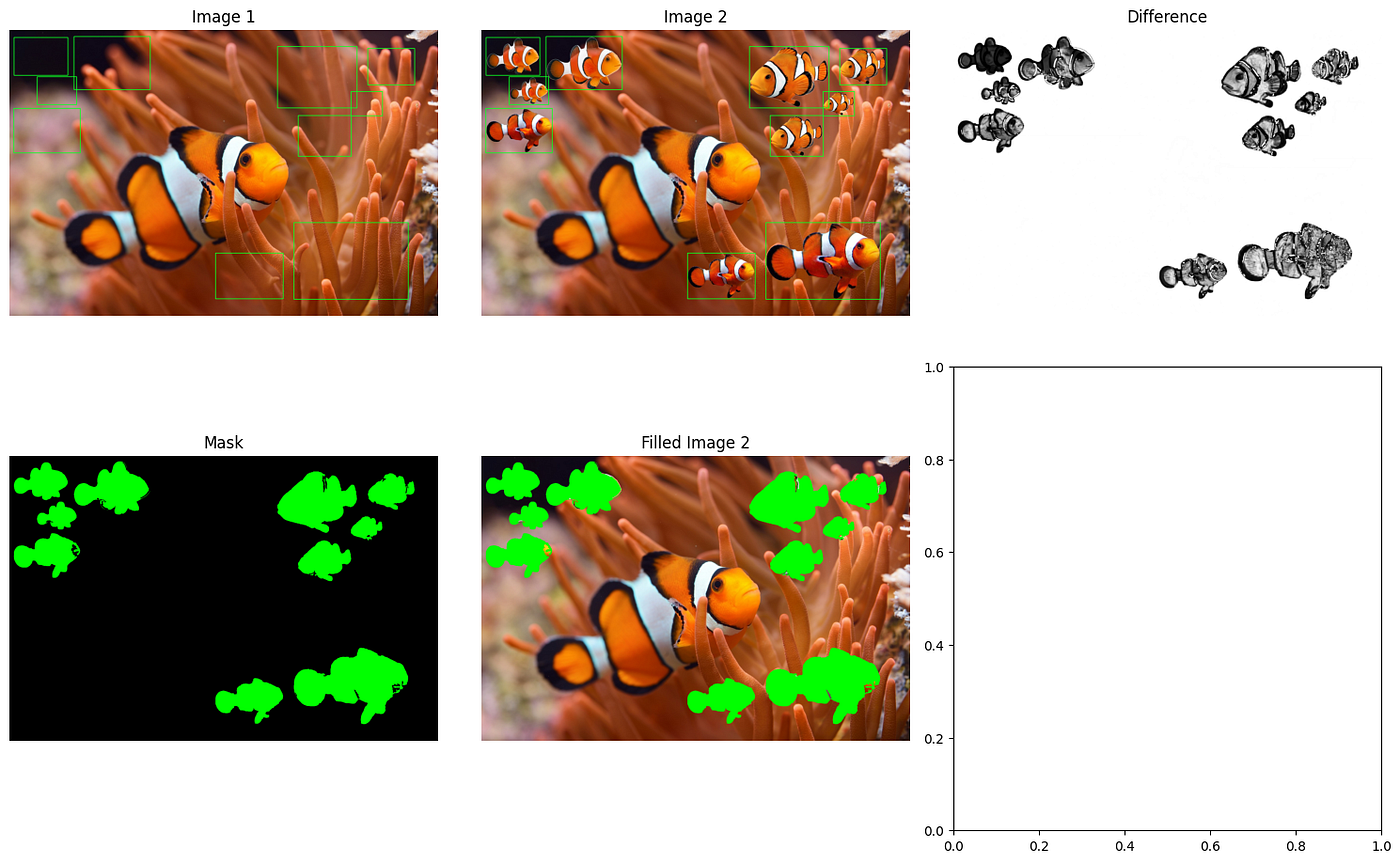
The Absolute Difference method is a pixel-wise comparison method. This method treats images as matrices and calculates the difference between the two matrices.
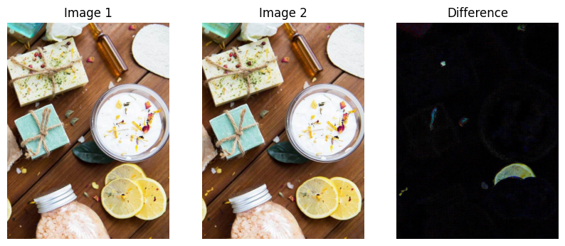
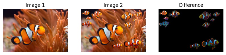
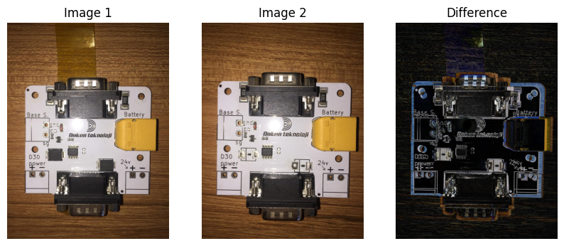
Method 6: Subtraction
Subtraction is a typical subtraction calculation. In OpenCV, subtraction is used for computing the absolute or relative difference between two images. It is often used to highlight areas and detect motion between two image frames. The difference between subtraction and absolute difference is that the former only provides the difference in intensity values without considering whether the difference is negative or positive, while the latter provides the absolute value of the difference.
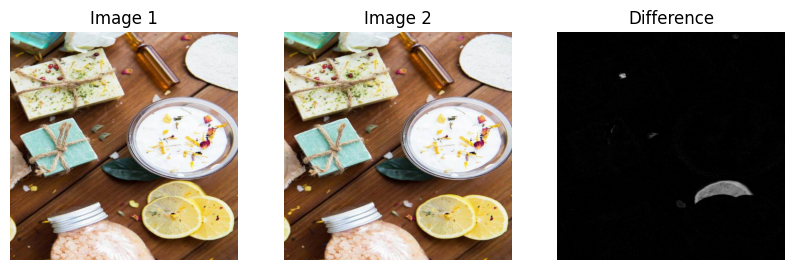
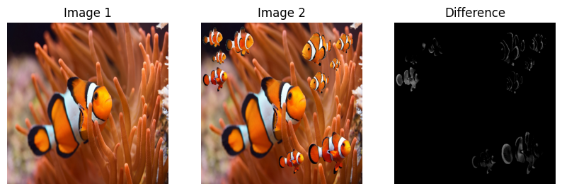
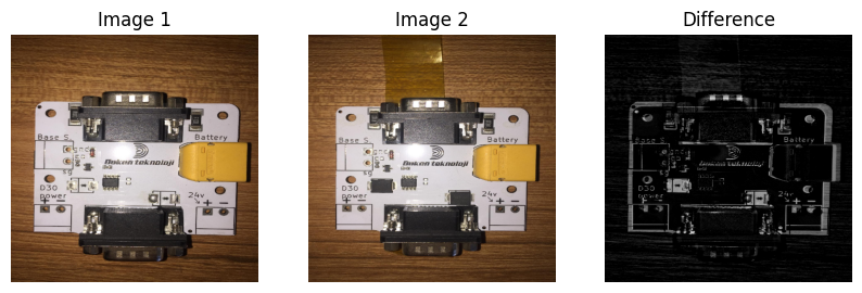
When Approaching the End
At the beginning of the paper, the main purpose was to compare two PCB cards, find differences, and highlight these points. During the research process, many resources on image comparison seemed perfect, as the examples used were similar to those in Photoshop, with no differences in lighting, scale, or size, and none of them were snapshots taken with a phone.
This was a challenging part of the project. In real life, people without a system cannot take two different versions of an object with the same brightness, scale, and size.
To carry out this project, I found PCB cards of the same size, but one had a missing component. I took pictures using an iPhone 6 and a flashlight. The collection part was done. After that, using Visual Studio Code, I started to write Python code. No matter how many times I tried, there would always be slight differences in size, scale, and lighting.
1st Step Importing Necessary Libraries
Importing necessary libraries
import numpy as np
import matplotlib.pyplot as plt
import cv2
import scipy.spatial import distance
2nd Step: Defining a function to resize images
This function is for making a little less complex comparison.
def resize_image(image, max_width, max_height):
    height, width = image.shape[:2] #(image.shape) == (height,width,number of color channel)
    scaling_factor = min(max_width / width, max_height / height)
    new_size = (int(width * scaling_factor), int(height * scaling_factor))
    return cv2.resize(image, new_size) #cv2.resize(image,(new_width,new_height))
3rd Step: Defining a function to merge close contours
One of the challenges at the end of the comparison process was the excessive number of contours on a single object. This function merges close contours. Note: I manually adjust the min_distance and max_distance parameters based on the results. There are two methods for merging close contours: one uses the numpy library to calculate distances between contours, and the other uses the scipy library.
# Way1
#-------------------------------------------------------------------------------------------

def merge_close_contours(contours, min_distance=0, max_distance=50):
    if len(contours) == 0:
        return []

    merged_contours = []
    centers = [cv2.moments(cnt) for cnt in contours]
    centers = [(int(M['m10'] / M['m00']), int(M['m01'] / M['m00'])) if M['m00'] != 0 else (0, 0) for M in centers]

    merged = [False] * len(contours)

    for i in range(len(contours)):
        if not merged[i]:
            current_merge = [contours[i]]
            for j in range(i + 1, len(contours)):
                if not merged[j]:

                    distance = np.sqrt((centers[i][0] - centers[j][0])**2 + (centers[i][1] - centers[j][1])**2)
                    if min_distance <= distance <= max_distance:
                        current_merge.append(contours[j])
                        merged[j] = True
            merged_contours.append(np.concatenate(current_merge))
            merged[i] = True

    return merged_contours

"""
# Way2
#-------------------------------------------------------------------------------------------

def merge_close_contours(contours, min_distance=20, max_distance=70):
    if len(contours) == 0:
        return []

    merged_contours = []
    centers = [cv2.moments(cnt) for cnt in contours]
    centers = [(int(M['m10'] / M['m00']), int(M['m01'] / M['m00'])) if M['m00'] != 0 else (0, 0) for M in centers]
    distances = distance.cdist(centers, centers, 'euclidean')

    merged = [False] * len(contours)

    for i in range(len(contours)):
        if not merged[i]:
            current_merge = [contours[i]]
            for j in range(i + 1, len(contours)):
                if not merged[j] and min_distance <= distances[i, j] <= max_distance:
                    current_merge.append(contours[j])
                    merged[j] = True
            merged_contours.append(np.concatenate(current_merge))
            merged[i] = True

    return merged_contours
"""
4rd Step: Defining a function prevent to overlapping boundries rectangles
When highlighting differences using rectangles, some of them overlap on the same component. To prevent this situation, I use another function.
def merge_overlapping_rectangles(rectangles):
    if len(rectangles) == 0:
        return []

    rectangles = [list(rect) for rect in rectangles]
    merged_rectangles = []

    while rectangles:
        rect1 = rectangles.pop(0)
        to_merge = [rect1]

        for rect2 in rectangles:
            if (rect1[0] < rect2[0] + rect2[2] and rect1[0] + rect1[2] > rect2[0] and
                rect1[1] < rect2[1] + rect2[3] and rect1[1] + rect1[3] > rect2[1]):
                to_merge.append(rect2)

        for rect in to_merge:
            if rect in rectangles:
                rectangles.remove(rect)

        x_min = min([rect[0] for rect in to_merge])
        y_min = min([rect[1] for rect in to_merge])
        x_max = max([rect[0] + rect[2] for rect in to_merge])
        y_max = max([rect[1] + rect[3] for rect in to_merge])

        merged_rectangles.append((x_min, y_min, x_max - x_min, y_max - y_min))

    return merged_rectangles
5th Step: Read, arrange size, aligment
I use the cv2.imread method for reading images. However, a significant challenge in real-life scenarios arises when slight differences exist between two pictures due to unstable arm positioning, lighting variations, and object distance. These factors can lead to poor results with traditional image comparison methods. To address this issue, I employ the ECC (Enhanced Correlation Coefficient) algorithm for alignment. This algorithm facilitates the alignment of two images by identifying the optimal transformation matrix. It iteratively adjusts this matrix towards an identity transformation, allowing detection of translations and small deformations between images.
imageA = cv2.imread('x1.png')
imageB = cv2.imread('x2.png')

# Check dimensions
h, w = imageA.shape[:2]
warp_matrix = np.eye(2, 3, dtype=np.float32)

# ECC algorithm for alignment
criteria = (cv2.TERM_CRITERIA_EPS | cv2.TERM_CRITERIA_COUNT, 5000, 1e-10)
(cc, warp_matrix) = cv2.findTransformECC(cv2.cvtColor(imageA, cv2.COLOR_BGR2GRAY), cv2.cvtColor(imageB, cv2.COLOR_BGR2GRAY), warp_matrix, cv2.MOTION_TRANSLATION, criteria)

# Align the second image
aligned_imageB = cv2.warpAffine(imageB, warp_matrix, (w, h), flags=cv2.INTER_LINEAR + cv2.WARP_INVERSE_MAP)

# Resize images to fit the screen
max_width = 800
max_height = 600
imageA_resized = resize_image(imageA, max_width, max_height)
aligned_imageB_resized = resize_image(aligned_imageB, max_width, max_height)
6th Step: Compare two images
After preparing the images, I compare them using the absolute difference method. Then, I apply a threshold to detect color changes (Note: the threshold parameter can vary depending on other references; I adjust it manually based on the results) and reduce noise using morphological operations. Finally, the average image is generated by averaging the two images at the end.
average_image = cv2.addWeighted(imageA_resized, 0.5, aligned_imageB_resized, 0.5, 0)

diff = cv2.absdiff(imageA_resized, aligned_imageB_resized)

# Apply a specific threshold value for detecting color difference (can be change for different images!!)
_, thresh = cv2.threshold(cv2.cvtColor(diff, cv2.COLOR_BGR2GRAY), 101, 255, cv2.THRESH_BINARY)

kernel = np.ones((5, 5), np.uint8)
thresh = cv2.morphologyEx(thresh, cv2.MORPH_OPEN, kernel)

# Find contours
contours, _ = cv2.findContours(thresh, cv2.RETR_EXTERNAL, cv2.CHAIN_APPROX_SIMPLE)

# Merging close contours
merged_contours = merge_close_contours(contours)
7th Step: Edge margin and calling merged rectangles
After displaying the differences, I encountered an error. The program was showing rectangles at the edges of the images due to poor snapshots. To prevent this, I implemented an edge margin to avoid displaying edge differences as rectangles.
edge_margin = 10  # to prevent edge contours

rectangles = []
for contour in merged_contours:
    if cv2.contourArea(contour) > 100 :
        x, y, w, h = cv2.boundingRect(contour)
        if x > edge_margin and y > edge_margin and x + w < imageA_resized.shape[1] - edge_margin and y + h < imageA_resized.shape[0] - edge_margin:
            rectangles.append((x, y, w, h))

merged_rectangles = merge_overlapping_rectangles(rectangles)

for (x, y, w, h) in merged_rectangles:
    cv2.rectangle(imageA_resized, (x, y), (x + w, y + h), (0, 255, 0), 2)
    cv2.rectangle(aligned_imageB_resized, (x, y), (x + w, y + h), (0, 255, 0), 2)
    cv2.rectangle(average_image, (x, y), (x + w, y + h), (0, 255, 0), 2)
8th Step: Showing Results
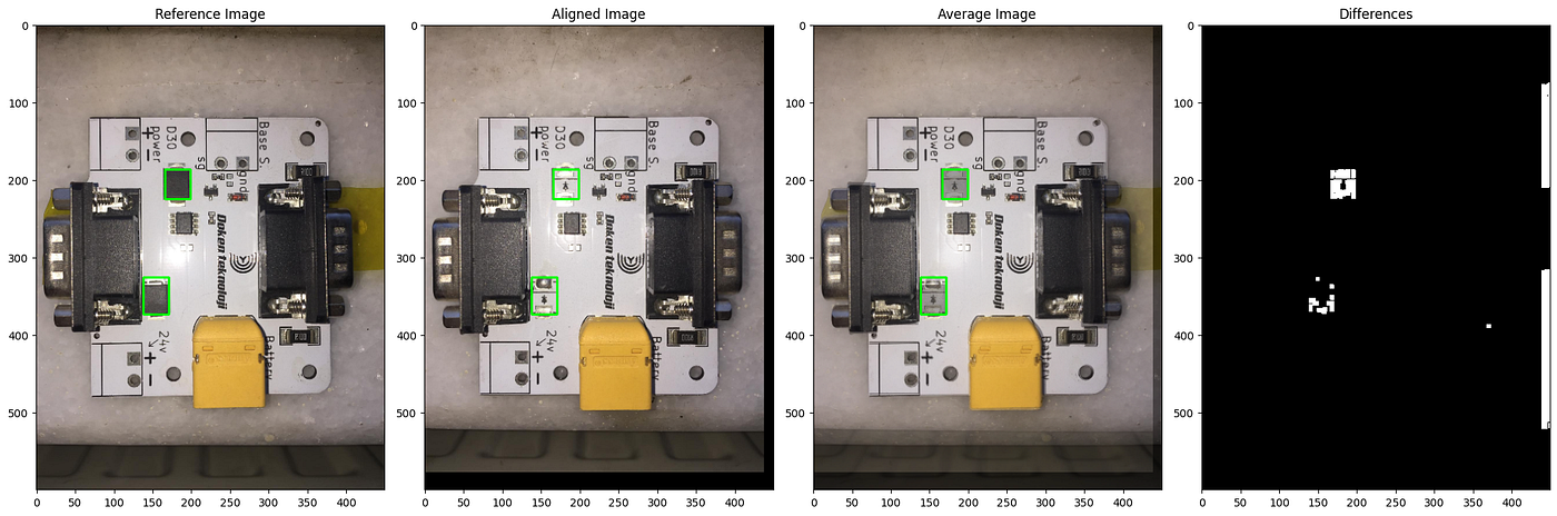
After calculating size, alignment, contours, and rectangles, we’ve reached the final step. To display the results, I use the matplotlib library. I created a 1x4 grid to show the results: the first figure displays the reference images, the second figure shows the test images aligned, the third figure shows the average image between the reference and aligned images, and the last figure shows the thresholded differences. To handle differences in color channels between OpenCV (which uses “BGR”) and matplotlib (which uses “RGB”), I performed color channel conversion as needed.
Let’s look at some results


Thank you for reading this paper. If it was helpful to you in any way, I would be glad.
I added end of the paper some resources and Github link of the project.
If you have any questions, feel free to contact me via email at: me.muhammed.dinc@gmail.com.
메타데이터
- post_id
- f2cd3376e89e
- slug
- pcb-card-comparison-for-finding-defects-it-includes-python-image-comparison-method-f2cd3376e89e
- url
- https://medium.com/@me.muhammed.dinc/pcb-card-comparison-for-finding-defects-it-includes-python-image-comparison-method-f2cd3376e89e
- canonical_url
- https://medium.com/@me.muhammed.dinc/pcb-card-comparison-for-finding-defects-it-includes-python-image-comparison-method-f2cd3376e89e
- author_url
- https://medium.com/@me.muhammed.dinc
- status
- ok
- fetched_at
- 2026-06-27 18:39:40