A Better Way to Understand Convolutions

Understanding convolutions using linear algebra

Image generated using DALL.E

Convolution is a mathematical operation that combines two functions to describe their overlap. It has many applications in statistics, signal processing, image processing, and computer vision. In deep learning, discrete convolutions play an important role in convolutional neural networks (CNNs). In this article, we will examine discrete convolutions closely and explore the intuition behind them using linear algebra. We will see a strong connection between discrete convolutions and cosine similarity.

All images with no source in the caption were created by the author.

Convolution and cross-correlation

The convolution of two functions f and g is defined as:

However, in data science and machine learning, we are more interested in discrete convolutions between two finite sequences. Let x be a sequence of numbers with P elements defined as:

And let w be a sequence defined as:

Please note that the number of elements in w is odd (2M+1), and the indices start from -M instead of zero. We write the indices of w this way because it simplifies the equations that define the convolution operation. The convolution of x and w denoted by *x*****w** is a sequence with P elements, and its i*th element is defined as:

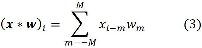
When using this equation, x and w are referred to as the signal and kernel, respectively. Let’s see an example. Suppose that:

Based on Equation 3, we can write:

Of course, there is a problem with these calculations. The signal doesn’t have any elements with indices 0 or 6. Hence, we assume that the signal is padded with zeros on both sides:

Now, the values of x at indices 0 and 6 are zero, and we can write:

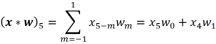
Figure 1 visually explains the convolution operation. We need to do the following steps: First, we flip the kernel sequence, which means we reverse it. We denote the flipped kernel with wᶠ. Then we place the kernel beside the signal so that the middle element of the kernel (w₀) is matched with the first element of the signal (x₀). Then we multiply each element of the kernel by the signal’s element on top of that and add all the products. The result is the first element of the convolution. To calculate the next element, we simply slide the kernel to the right by one element and repeat the same operations.

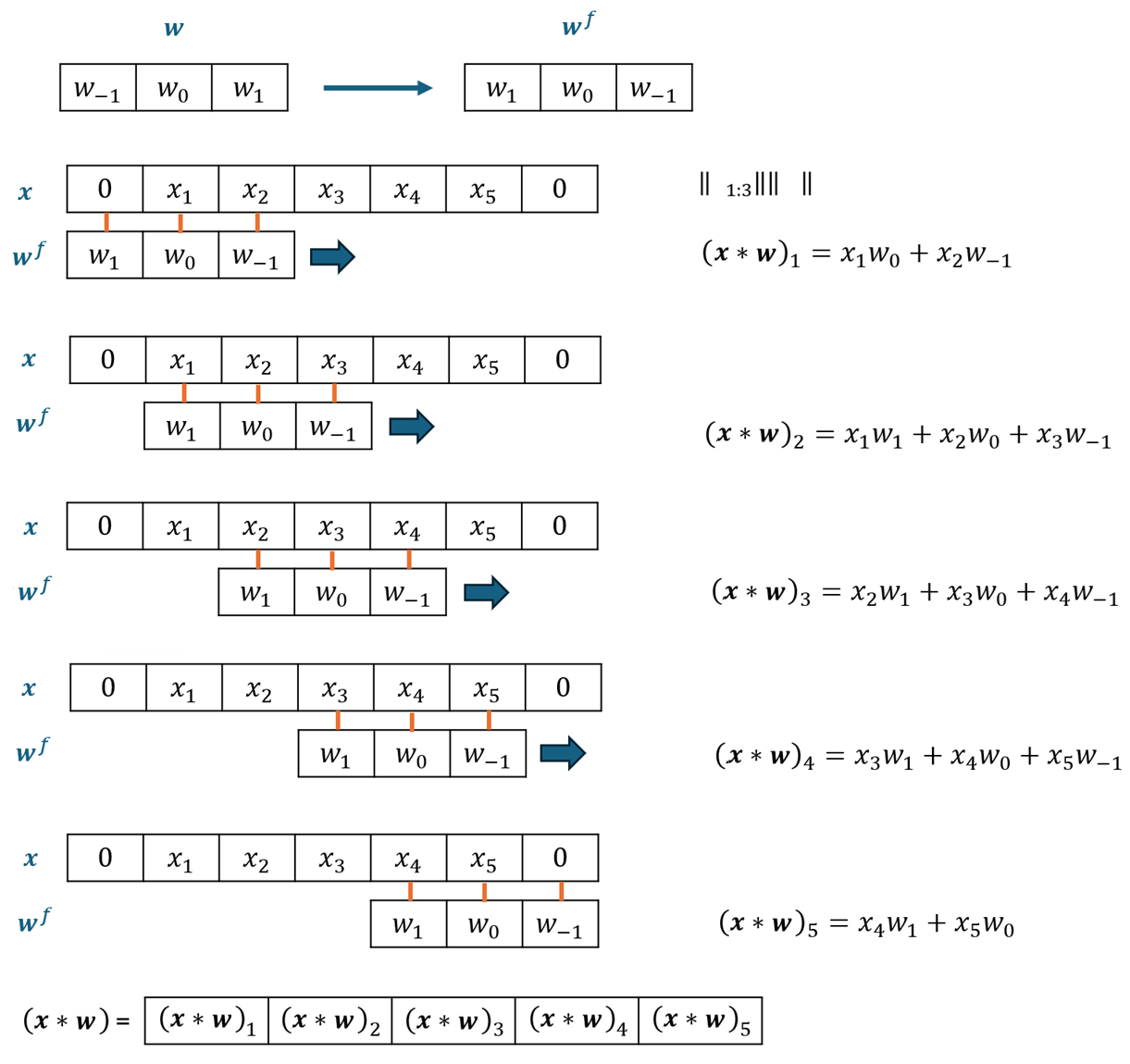
Figure 1

There is another operation known as cross-correlation that is closely related to convolution. Suppose we have the same signal (x) and kernel (w) defined in equations 1 and 2. The cross-correlation of x and w, denoted by C(x,w), is a sequence with P+1 elements, and its ith element is defined as:

Figure 2 visually explains the cross-correlation operation. Here, we use the same signal and kernel shown in Figure 1.

Figure 2

As you see, the operation is similar to a convolution. The only difference is that the kernel is not flipped anymore. If we compare a kernel with its flipped version, we can write:

Figure 3 shows an example of this relationship.

Figure 3

Now we can use this definition to write:

So we have:

Similarly, we can write:

This means that we can convert a convolution to cross-correlation and vice versa by just flipping the kernel. Now here is the question. What are these operations doing from a mathematical point of view? In the next section, we answer this question.

This means that we can convert a convolution to cross-correlation and vice versa by simply flipping the kernel. Now here is the question. What are these operations accomplishing from a mathematical perspective? In the next section, we will address this question.

Cosine similarity

Cosine similarity measures the similarity between two non-zero vectors by calculating the cosine of the angle between them. It is a mathematical concept widely used in data analysis and machine learning. Cosine similarity is by definition the cosine of the angle between the vectors and can be calculated by dividing the dot product of the vectors by the product of their lengths (Figure 4). Let u and v be two vectors with n elements:

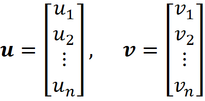
The cosine similarity between u and v is defined as:

where u.v is the dot product of u and v, and is defined as:

||u|| and ||v|| denote the length of u and v respectivly. The length of a vector like u is defined as:

Figure 4

The cosine similarity is always between -1 and 1. Many machine learning applications require that the vector components be nonnegative. In that case, the cosine similarity is limited to the interval [0, 1]. If the vectors point in the same direction, the angle between them is zero, and cos(0)=1. Thus, when the vectors point in the same direction, their cosine similarity is at its greatest. Let’s take an example. Suppose we have the following vectors:

Since these vectors have 4 elements, we cannot show them in a 3-D space. Instead, we use a line plot to visualize them. In this line plot, each component of a vector is represented by a dot. The x-axis represents the index of the components, and the y-axis represents their values. Using this method, we can visualize a vector with any number of components. For example, the vector w can be shown using the following plot:

Figure 5

Listing 1 plots the vectors u, v, w and r and calculates the cosine similarity between each pair of them. The result is shown in Figure 6.

# Listing 1

import numpy as np
import matplotlib.pyplot as plt
from numpy.linalg import norm

w= np.array([2,3,2,4])
u=2*w
v= w+1
r = np.array([4,2,6,1])

cos_sim_wu = np.round(np.dot(w, u)/(norm(w)*norm(u)), 4)
cos_sim_wv = np.round(np.dot(w, v)/(norm(w)*norm(v)), 4)
cos_sim_wr = np.round(np.dot(w, r)/(norm(w)*norm(r)), 4)

fig, axes = plt.subplots(1, 3, figsize=(10, 3))
ind = [1,2,3,4]
axes[0].plot(ind, w, marker="o", label="w")
axes[0].plot(ind, u, marker="o", label="u")
axes[1].plot(ind, w, marker="o", label="w")
axes[1].plot(ind, v, marker="o", label="v")
axes[2].plot(ind, w, marker="o", label="w")
axes[2].plot(ind, r, marker="o", label="r")

for ax in axes:
    ax.set_xlabel("Component index", fontsize=12)
    ax.set_ylim([1,9])
    ax.legend(fontsize=11)

axes[0].set_ylabel("Component value", fontsize=12)
axes[0].set_title(rf"$cos(\theta)=${cos_sim_wu}", fontsize=14)
axes[1].set_title(rf"$cos(\theta)=${cos_sim_wv}", fontsize=14)
axes[2].set_title(rf"$cos(\theta)=${cos_sim_wr}", fontsize=14)

plt.show()

Figure 6

The vectors u and w have the same direction since u=2w. Hence, they have the maximum cosine similarity of one. The vectors r and w have the least similarity and the lowest cosine similarity. It is interesting to note that though the line plot of the vectors v and w shows a similar trend (since v=w+1), their cosine similarity is less than 1. Additionally, u and w have the maximum cosine similarity, but the trend of their line plots looks different. This is just an illusion, and if we plot them separately with different scales, we see the line plots have the same trend. This is demonstrated in Figure 7.

Figure 7

Cosine similarity is a powerful concept, but it can only be used for two vectors with the same number of components. What if we want to compare the similarity of a vector to another one with more components? For example, suppose that we want to find the similarity between the vectors w and x defined as:

Here, we cannot calculate the cosine similarity of x and w. Instead, we can break x into smaller pieces where each piece has the same length as w. Then we can calculate the cosine similarity between each piece and w as shown in Figure 8.

Figure 8

In this figure, *x_m:n denotes a slice of the vector x* that contains the elements xm to xn:

Hence, we can write each cosine similarity component as:

Please note that we can also show a vector as a sequence. Therefore, the vectors

can also be written as sequences

since they both represent an ordered set of numbers. So, we can still use the same equations to calculate the dot product, length and cosine similarity for them. In fact, it doesn’t matter if we think of the signal and kernel as vectors or sequences. Now let’s see an example. Listing 2 calculates the cosine similarity between the sequences

# Listing 2

w = np.array([1,3,2])
x = np.array([5,1,3,2,5,0,4,12,8,0,1])

x_padded = np.pad(x, (1, 1), 'constant')
result = np.zeros(len(x)) 
for i in range(0, len(x_padded)-2):
    result[i] = np.dot(x_padded[i:i+len(w)], w)
    result[i] /= np.linalg.norm(x_padded[i:i+len(w)])*np.linalg.norm(w)
np.round(result, 2)

array([0.89, 0.63, 1. , 0.82, 0.84, 0.54, 0.76, 1. , 0.67, 0.33, 0.8])

Figure 9 visualizes the resulting sequence (the black line plot). As this figure shows, two slices in x have the maximum similarity with w and result in a cosine similarity of 1. These slices are

which is equal to w, and

that is equal to 3w.

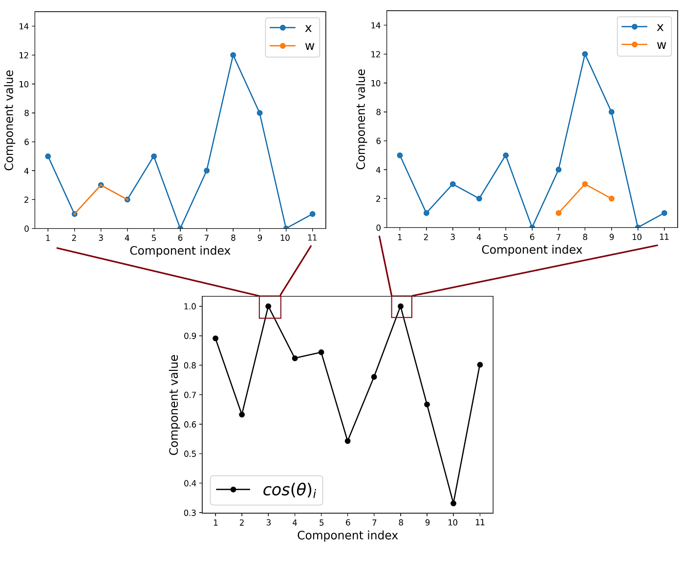
Figure 9

Now, let’s look at the connection between the cosine similarity and cross-correlation. Looking at Equation 5, we see that removing the denominator yields the cross-correlation formula (Equation 4). In fact, the cross-correlation is simply the dot product of the kernel and a slice of the signal. Hence, we can write:

So, cross-correlation can be defined as the cosine similarity between a slice of the signal and the kernel multiplied by their respective lengths. But why do we apply this multiplication instead of simply using the cosine similarity?

First, let’s focus on the length of the kernel (||w||). The length of the kernel doesn’t depend on i, which means that it remains the same for all the components of the cosine similarity. Hence, when we multiply the components of the cosine similarity by ||w||, it only acts as a scale factor and does not alter the ratio of one component to another.

Listing 3 plots the cosine similarity between the vectors x and w (defined in Listing 2). It also plots the cosine similarity multiplied by the length of w. The result is shown in Figure 10. As you see, ||w|| only acts as a scale factor and doesn’t change the trend of the cosine similarity line plot. As mentioned before, there are two slices in x that have the maximum cosine similarity with *w (x*_2:4 and x_7:9). The cosine similarity of these slices is 1. When we multiply the cosine similarity by ||w||, these slices still have the highest values. Their value has now been scaled to ~3.74.

# Listing 3

w = np.array([1,3,2])
x = np.array([5,1,3,2,5,0,4,12,8,0,1])

x_padded = np.pad(x, (1, 1), 'constant')
result = np.zeros(len(x)) 
for i in range(0, len(x_padded)-2):
    result[i] = np.dot(x_padded[i:i+len(w)], w)
    result[i] /= np.linalg.norm(x_padded[i:i+len(w)])*np.linalg.norm(w)

cosine_sim  = result
cosine_sim_times_w  = result * np.linalg.norm(w)
cross_corr  = np.correlate(x, w, mode='same') 

fig, axes = plt.subplots(1, 3, figsize=(10, 3))
ind = range(1, len(result)+1)
axes[0].plot(ind, result, marker="o")
axes[1].plot(ind, cosine_sim_times_w, marker="o")
axes[2].plot(ind, cross_corr , marker="o")

for ax in axes:
    ax.set_xlabel("Component index", fontsize=13)
    ax.set_xticks(np.arange(1, 12))

axes[0].set_ylabel("Component value", fontsize=13)
axes[0].set_title(r"$cos(\theta)_i$", fontsize=14, pad=10)
axes[1].set_title(r"$||w||cos(\theta)_i$", fontsize=14, pad=10)
axes[2].set_title(r"$C(x,w)_i=$"r"$||x_{i-M:i+M}||.||w||cos(\theta)_i$",
                  fontsize=14, pad=10)

plt.show()

Figure 10

Listing 3 also plots the cross correlation of x and w, which is equal to the cosine similarity multiplied by ||*w|| and the length of each slice of x*. Please note that when we add the length of the slices, the slice x_7:9 becomes much more important than x_2:4. That is because the length of the latter is much greater than that of the former. Now x_7:9 has the maximum cross-correlation with the kernel, but the cross-correlation of x_2:4 is a relatively small number. Hence, we conclude that what cross-correlation measures is not just the similarity between the signal and the kernel. It also considers the length of the signal.

Signal refers to the meaningful, relevant information that you are trying to detect or measure from a set of data. Essentially, the signal is what you want to capture or analyze. On the other hand, noise refers to the irrelevant, random, or unwanted data that interferes with the signal or obscures it. Consider a radio as an example. The signal is the music you want to hear, while the noise is static and interference from other channels. In practice, signals are almost always accompanied by some level of noise. Hence, in many fields like data science and machine learning, distinguishing the signal from the noise is critical for effective data analysis, modelling, and decision-making.

The signal can be separated from noise based on the signal strength. In the cross-correlation formula, the length of a slice of x represents its strength at that region. Though we call the sequence x the signal, it can also be accompanied by noise. So, when a local slice of x has a relatively low strength, we can assume that it is mostly noise, and its similarity with the kernel can be a random event which shouldn’t be captured. Cross-correlation evaluates a signal’s strength as well as its similarity to the kernel. Pure similarity is insufficient for obtaining a high cross-correlation value; the signal in that area should also be relatively strong.

Figure 11 shows another example. Here, a weak and noisy slice of the signal has the maximum similarity with the kernel, but its cross-correlation component is low. On the other hand, another slice has a smaller cosine similarity, but its much greater strength results in a greater cross-correlation.

Figure 11

2D cross-correlation and convolution

So far, the signal and kernel were one-dimensional sequences, however, we can also have 2 dimnesional signals and kernels. Let the signal be a P × K matrix defined as:

We also defined the kernel with the following matrix:

The cross correlation of X and W is a P × K matrix whose entries are defined as follows:

As an example, let’s calculate the cross-correlation of the following signal and kernel:

Figure 12 shows the first step of the calculations. Like 1D cross-correlation, we need to pad the signal matrix with zeros. Then we place the kernel on the top-left corner of the padded signal and compute the product of the mutually overlapping elements of the signal and the kernel, and calculate their sum. The result will be the first entry of the output pixel at that particular location.

Figure 12

The kernel slides across the signal one pixel at a time to calculate the other entries of the cross-correlation matrix (Figure 13).

Figure 13

Let’s take a look at the connection between the 2D and 1D cross-correlation. To understand this connection, we need to flatten the kernel and each slice of the signal on which the kernel is applied. Flattening a matrix transforms it into a one-dimensional vector (or sequence). Think of it like stacking rows of the matrix on top of each other to form a single long row. For example, if we flatten the kernel

results in the vector

Figure 14 shows the calculations to obtain the first entry of the cross-correlation matrix. We flatten the kernel and the corresponding slice of the signal and denote them by w’ and x’. The entry of the cross-correlation matrix is simply the dot product of x’ and w’. Remember that we calculated the 1D cross-correlation in the same way (Equation 6). Hence, we can use the same interpretation that we had for 1D cross-correlation. If we think of the kernel and each slice of the signal as flattened vectors, the cross-correlation between them is simply their dot product and is proportional to their cosine similarity time the strength of the slice of signal (Figure 14).

Figure 14

Next, we look at 2D convolution. Let X and W be the same signal and kernel defined in Equation 8. The convolution of X and W is a P × K matrix whose entries are defined as follows:

Let’s see how this equation is related to the cross-correlation formula in Equation 7. We defined a flipped 2D kernel using the following equation:

For example, if we have:

Then, flipping W will result in this matrix:

Now, using this definition,n we can write:

So, it follows that:

which can also be written as:

This means that we can convert a convolution to cross-correlation and vice versa by just flipping the kernel. Remember that we obtained a similar relationship between the 1D convolution and cross-correlation. Figure 15 gives a visual demonstration of the steps to calculate the convolution of the signal and the kernel given in Equation 8.

Figure 15

But why do we need Equation 9 to flip the kernel? Remember that for 1D signals and kernels, each component of the cross-correlation is the dot product of the kernel and the corresponding slice of the signal (refer to Figure 2). In case of convolution, we only need to flip the kernel and then calculate the dot product (Figure 1). For the 2D case, each component of the cross-correlation is the dot product of the flattened kernel and the flattened slice of the signal (Figure 14). Equation 9 simply flips the flattened kernel for us. This is demonstrated with an example in Figure 16.

Figure 16

Here we flattened the kernel (W) and flipped the kernel (*Wᶠ) into the 1D vectors (or sequences) w*’ and *wᶠ ’, and we can see that wᶠ ’ is the same as flipped w*’.

Valid versus exact operations

So far, we padded the signal before applying the kernel to that for both cross-correlation and convolution. An exact convolution (or cross-correlation), also known as the same convolution (or cross-correlation), uses padding to ensure the output size matches the input size. In all the examples, the size of the output is equal to that of the signal. For example, in Figures 13 and 15, the signal was a 4 × 4 matrix, and both the cross-correlation and convolution matrices were also 4 × 4. We can also apply the kernel without padding the signal, and this is called a valid convolution (or cross-correlation), which results in a smaller output compared to the input signal. Figure 17 shows a valid cross-correlation on the same kernel and signal used in Figure 13. The signal is a 4 × 4 matrix, but since no padding is used, the cross-correlation matrix is 2 × 2.

Figure 17

Convolutional neural networks

A Convolutional Neural Network (CNN) is a type of artificial neural network that’s particularly designed for image processing and recognition tasks. It is described as an architecture that uses the convolution operation to extract features from input data, like images, and then uses these extracted features to classify or recognize objects within the image.

We observed that convolution and cross-correlation are two distinct operations that can be converted into one another by flipping the kernel. However, in the context of deep learning, it is common to refer to both operations as a convolution, which can lead to confusion. In fact, most convolution operators in deep learning are implemented as cross-correlations, though they are called a convolution. For example, in a convolutional neural net, we use cross-correlation operations to extract features, not convolutions. Looking at the PyTorch manual, we see that the Conv1dand Conv2d (https://pytorch.org/docs/stable/generated/torch.nn.Conv1d.html and https://pytorch.org/docs/stable/generated/torch.nn.Conv2d.html) are called the classes that apply a 1D or 2D convolution over the input signal, but as the manual explains, both are indeed valid cross-correlation operators for the input signal.

In this article, we explained the intuition behind convolution and cross-correlation using linear algebra. We saw the delicate connection between the cross-correlation and convolution operations. A cross-correlation tries to measure the cosine similarity between a kernel and the slices of the signal, which have the same size as the kernel. However, it also takes into account the strength of each slice to remove the exclude the noisy slices. A convolution operation is the same as a cross-correlation with a flipped kernel.

[embed]Get an email whenever Reza Bagheri publishes. Get an email whenever Reza Bagheri publishes. By signing up, you will create a Medium account if you don't already have…reza-bagheri79.medium.com

I hope you enjoyed reading this article. Please let me know if you have any questions. If you find my articles helpful, please follow me on Medium.