Save Cloud Bills By Optimizing Spark Workloads

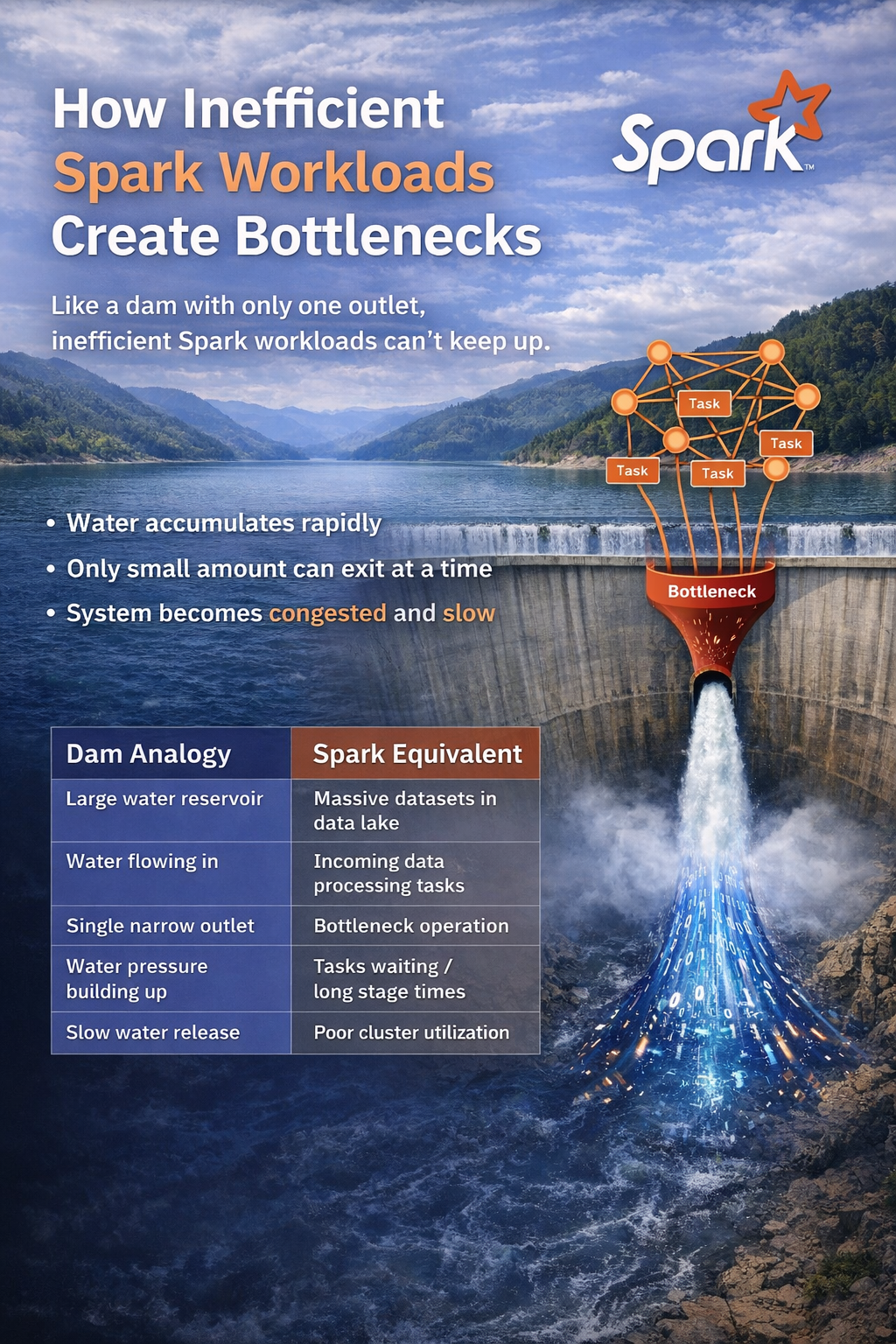
Building unoptimized Spark workloads is like constructing a dam reservoir with only one outlet. While it may hold enormous power, it creates bottlenecks and overhead, leading to poor efficiency.

In this blog, I will walk you through some optimization techniques. If you are visiting for the first time and would like to gain a basic foundational understanding of Spark, you can access my previous blog here:

To add more credibility to what i am sharing in this article, I would like to let you know I am spark certified. here is my certification URL:

A common misconception among Spark beginners is that using Pandas is always discouraged. While this is true in many large-scale data processing scenarios, there are situations where using Pandas can be practical. For example, if the dataset is smaller than 20 MB, it may not be necessary to spin up all the executors in a Spark cluster. Since Pandas runs on a single node, it avoids the overhead of starting multiple executors, leading to faster computation and more efficient resource utilization.

Partition Pruning

Partition pruning in Apache Spark is a technique that skips unnecessary partitions and reads only the relevant data based on partition filters. This reduces the amount of data scanned, improves performance, and lowers compute costs. For example, if you have a large dataset that is frequently queried by year, partitioning the dataset by year can significantly reduce scan time because Spark will read only the required partition.

In Apache Spark, partitioning strategies are crucial because they directly affect parallelism, query performance, and shuffle costs. An optimal partitioning strategy ensures that data is evenly distributed across executors and enables optimizations such as partition pruning.

1. Partition by Frequently Filtered Columns.
2. Avoid High Cardinality Columns.
3. Avoid Very Low Cardinality Columns
4. Target Optimal Partition Size (100 mb — 1 gb per partition)
5. . Repartition Before Writing
6. Use Coalesce for Reducing Partitions
7. Consider Query Patterns (Always design partitions based on how data is queried, not how it is stored.)
8. Use Multi-Level Partitioning (Like ex: Year, Month, Day)

Always try to optimize Number of Partitions : Cluster performance depends heavily on partition count relative to CPU cores.

Rule of thumb: Total partitions = 2–4 × total cluster cores

Join Strategies

Joins are one of the most compute-intensive operations in Apache Spark. In many real-world pipelines, joins consume the majority of execution time and cluster resources. Let’s understand why joins are expensive in Spark.

Data Shuffling (Main Reason) : Most joins require data to be redistributed across the cluster, a process called shuffle. Data Skew Problems (If one key appears very frequently then one partition will be overloaded. Memory Pressure : Join operations often require holding large datasets in memory.

Join strategies in Apache Spark determine how Spark physically executes joins, balancing shuffle cost, memory usage, and dataset size to achieve the best performance.

In Apache Spark, join strategies define how Spark physically executes a join operation between two datasets. The optimizer in Spark (called the Catalyst Optimizer) automatically chooses the best strategy based on data size, partitioning, and configuration.

The main join strategies in Spark are:

1. Broadcast Hash Join
2. Shuffle Hash Join
3. Sort Merge Join
4. Broadcast Nested Loop Join
5. Shuffle Replicate Nested Loop Join.

Broadcast Hash Join

If one table is small enough, Spark broadcasts it to all executors so that each partition of the large table can join locally. This is how it works

1. Small table is copied to all executors.
2. Large table remains partitioned.
3. Each executor performs the join locally.

Shuffle Hash Join:

Both tables are shuffled based on the join key, then Spark builds a hash table on one side.

1. Shuffle both datasets
2. Partition by join key
3. Build hash table for smaller partition
4. Probe with the other dataset

In a Shuffle Hash Join in Apache Spark, Spark joins two large datasets by redistributing the data across the cluster based on the join key.

First, Spark shuffles both datasets, meaning rows are moved between executors so that rows with the same join key end up in the same partition. Once the shuffle is complete, each partition contains the matching keys from both datasets.

Next, within each partition, Spark selects the smaller dataset and builds an in-memory hash table using the join key. The other dataset is then scanned row by row, and Spark quickly checks the hash table to find matching records.

This approach is efficient because hash table lookups are very fast, but it can still be expensive since the shuffle phase involves network data transfer and disk I/O.

In short: a Shuffle Hash Join shuffles both datasets by the join key, builds a hash table from the smaller side in each partition, and probes it with the other dataset to produce the final join results.

Sort Merge Join

A Sort Merge Join is a distributed join strategy used for large datasets. It works in three main steps:

1. Shuffle — Spark redistributes both datasets across the cluster so that all rows with the same join key end up in the same partition. This ensures matching keys can be joined locally.
2. Sort — Each partition is sorted by the join key. Sorting allows Spark to scan both datasets sequentially, making the join efficient even for very large partitions.
3. Merge — Spark walks through the sorted partitions, comparing keys to produce the final joined rows. Matching keys are merged, and unmatched rows are ignored or included depending on the join type.

Why it’s used for large datasets:

• No need for a table to fit in memory (unlike hash joins).
• Handles big tables efficiently by processing partition by partition.
• Scales well across many executors and partitions.

In short: A Sort Merge Join shuffles, sorts, and merges large datasets by the join key, making it scalable and memory-efficient for distributed big data processing

Broadcast Nested Loop Join

This is used when:

• The join condition is not an equality condition (e.g., > , <, !=)
• Or when performing cross joins
• And one table is small enough to broadcast

Unlike hash or sort-merge joins, Spark cannot use a hash table or sorted merge for these conditions. Instead, it performs a nested loop join, comparing each row of the larger dataset with all rows of the smaller dataset.

• Spark sends a copy of the small table to all executors. Scan the large table partition by partition
• For each row in the large table, Spark checks every row in the broadcasted small table against the join condition.
• Rows that satisfy the join condition are included in the final output.

Shuffle Replicate

• Used for: Joins with complex or non-equality conditions where hash joins or sort-merge joins are not applicable.
• When one table cannot be broadcast (too large) but the join condition still requires a nested loop comparison.

It’s a rarely used join strategy because it is very compute-intensive. This is how it works

Replicate the smaller table across partitions

• Unlike broadcast joins, replication happens per partition during a shuffle.
• Each partition of the large table receives all rows from the smaller table relevant to that partition.

Scan the large table partition by partition

• For each row in the large table, Spark compares it with all replicated rows from the smaller table according to the join condition.
• Rows that satisfy the join condition are included in the final result.

Here’s a short 3-line guide for partition usage in Spark joins:

1. Broadcast Hash Join: Use when one table is small enough to fit in memory; Spark broadcasts the small table to all partitions of the large table.
2. Shuffle Hash Join: Use when both tables are medium-sized; Spark hash-partitions both tables by join key and builds a hash table per partition.
3. Sort Merge Join: Use for very large tables where neither fits in memory; Spark shuffles and sorts partitions by join key, then merges them sequentially.

Optimal DAGs

Optimizing DAGs (Directed Acyclic Graphs) in Apache Spark is one of the most effective ways to reduce compute cost, runtime, and resource usage. When DAGs are inefficient, Spark may perform unnecessary shuffles, re-computations, and large stage executions, which increases cluster cost.

Minimize Shuffles, Use Proper Partitioning, Cache Intermediate Data Wisely, Filter Early (Predicate Pushdown) Always reduce dataset size as early as possible in the DAG.

read → join → filter

read → filter → join

Cluster configurations

Optimizing cluster configuration in Apache Spark is critical for reducing compute cost and improving DAG execution performance. Many Spark jobs become expensive not because of bad code, but because the cluster resources are incorrectly sized or configured. One of the biggest mistakes is over-allocating executors. Make sure to allocate the right configurations using the parameters spark.executor.instances, spark.executor.cores spark.executor.memory

Enable Dynamic Resource Allocation which automatically adds/removes executors based on workload by using the parameters below:

spark.dynamicAllocation.enabled=true spark.dynamicAllocation.minExecutors=2 spark.dynamicAllocation.maxExecutors=50 spark.dynamicAllocation.initialExecutors=5

Memory Management Optimization

Memory configuration is important to prevent: Out of Memory errors, Disk spilling, Long GC pauses using the parameters below:

spark.executor.memory spark.executor.memoryOverhead spark.memory.fraction

AQE dynamically adjusts the execution plan during runtime.

Optimize Driver Configuration

The driver coordinates the DAG and schedules tasks. Bad driver configuration leads to: Task scheduling delays, Driver memory crashes

Optimize Shuffle Configuration

Shuffles are expensive operations. So make sure to optimize using the sample paramters below as per requirements.

spark.shuffle.file.buffer=1m spark.reducer.maxSizeInFlight=48m spark.shuffle.compress=true spark.shuffle.spill.compress=true

Golden Rule for Spark Cluster Optimization is to balance between CPU cores, Memory, Partitions, Executors.

Goal is to Keep all cores busy with minimal memory pressure and minimal shuffle overhead.

Storage Formats

Always prefer columnar formats over row-based formats. Why columnar formats are better because of Column pruning, predicate pushdown, better compression, faster analytics queries. Enable Compression which reduces reduces storage and network transfer. Spark supports compressions like Use CaseSnappyFast compression, GzipHigh compression, LZ4Balanced

Optimize File Sizes (Avoid Small Files Problem)

Small files create metadata overhead and slow down jobs Golden Rule for Spark Storage Optimization Store less data, scan less data, and read only what you need.

Delta Lake Optimizations

Optimizing tables in Delta Lake (which runs on Apache Spark) focuses on reducing file scans, improving data skipping, and maintaining efficient storage layout. These optimizations significantly improve query performance and reduce compute cost.

OPTIMIZE (File Compaction)

Delta tables often suffer from the small files problem, especially with streaming or frequent writes.

Small files cause:

• High metadata overhead
• Slow reads
• Poor query performance

Benefits:

• Faster queries
• Less metadata scanning
• Reduced I/O

Z-Ordering (Data Clustering)

Z-ordering improves data skipping by colocating related data.

Example: OPTIMIZE sales_table ZORDER BY (customer_id);

• Rows with similar customer_id values are stored close together.

Partition Optimization, Delta tables support partitioning.

Example CREATE TABLE sales USING DELTA PARTITIONED BY (year, month)

Only the 2025 partition will be scanned.

Schema Optimization

Delta supports schema evolution. Best practices include:

• Avoid frequent schema changes
• Use consistent data types
• Maintain schema governance

This prevents unnecessary metadata growth.

Optimize Write Operations

When writing large datasets, avoid generating too many small files. Benefits: Balanced file sizes and improved read performance.

The golden rule for Delta Lake optimization is to compact files, cluster frequently queried data, and remove unused storage.

These optimization techniques have the potential to significantly reduce cloud compute costs while allowing Spark to run more efficiently. If you’ve made it to the end of this blog, I hope you’ve learned something valuable and enjoyed reading it. Have a wonderful day. Thanks.