Classical physics may emerge spontaneously from quantum

How many of you know the difference between quantum and classical physics? Raise your hands.

If I were to call on you to define it, what would you answer?

The Infinite Universe is a reader-supported publication. To receive new posts and support my work, consider becoming a free or paid subscriber.

The old-school answer might be that classical physics is the limit as Planck’s constant goes to zero. But that isn’t really an answer. It’s just a mathematical statement.

Another might be that it is when Heisenberg’s uncertainty vanishes (which is a consequence of the first answer). In this case, it is possible to know the exact position and velocity of a particle at the same time.

That answer is closer to the truth, but perhaps it isn’t the fullness of the truth.

A third answer is that, whereas in classical physics you can predict the past and future of a system precisely, provided you know its exact state, in quantum mechanics, you can at best predict probabilities.

This is getting closer, but it is still missing an ingredient. I could say the same thing about a classical stochastic process, and I wouldn’t get quantum mechanics.

So what is the answer? What is my answer?

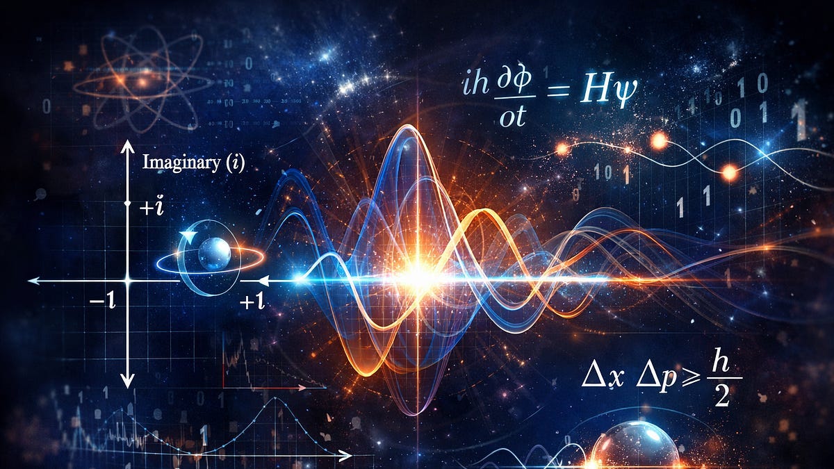
My answer is that in quantum mechanics, there exists an entity called a wavefunction. This is a wave-like object having both amplitude and phase. Wavefunctions combine in ways that let you add them together to represent new wavefunctions, which are called superpositions. These wavefunctions evolve according to an equation called Schrodinger’s equation that evolves the wavefunction forward in time. The probability that you will find a particle in a particular state when you measure it is equal to the square norm of the wavefunction (which is the wavefunction times its complex conjugate).

I like this answer not because it is the most complete (after all, I have just established that wavefunctions exist ontologically, which is disputed, and I have completely ignored other mathematically formalisms such as the Heisenberg picture and even time-independent Schroedinger’s) and not because it is the easiest to understand, but because it is the most complete answer that is easy to understand.

There are a few important points here as to why I think that: (1) quantum mechanics is weird, and one of the easiest ways to understand why it is weird is to recognize that wavefunctions are not probabilities but rather like square roots of probabilities. They contain not only amplitude, which is what determines the probability, but also phase information. Therefore, they combine like waves, interfering with one another as well as constructively adding together. This is exactly why you can have effects like entanglement, where one particle appears to affect another distant particle instantaneously. This only happens because wavefunctions are waves and not probabilities. (2) Squared wavefunctions are probabilities. This is important and has a name: the Born rule, after quantum mechanics pioneer Max Born. Without this rule, there is no quantum mechanics. And finally (3) Schroedinger’s equation evolves wavefunctions forward in time so wavefunctions are not static objects but they move and change.

Classical mechanics, on the other hand, has no wavefunctions. It represents particles purely as having position, velocity, and so on in a definite way, but more importantly, even when particles are represented probabilistically, as in Brownian motion, for example, where they are jostled around by molecules, those probabilities do not combine like waves. There is no weirdness.

Potentially, if we understood quantum mechanics better and where it comes from, we could come up with a shorter and more intuitive answer, but I’m not so sure. Most of the various interpretations that we are aware of, when they are explained to the layperson, ignore the phase information in the wavefunction entirely. The Many Worlds interpretation allows multiple realities to coexist, but this is just ordinary probability. It doesn’t explain how those probabilities got there in the first place! It was through the summation of complex numbers, not classical probabilities.

I guess I’m trying to hammer home here that quantum mechanics is not just classical mechanics with probabilities. That is classical stochastic mechanics. Because of the phase information in the wavefunction, quantum mechanics becomes something far weirder. We can only understand this if we think of all reality in terms of waves.

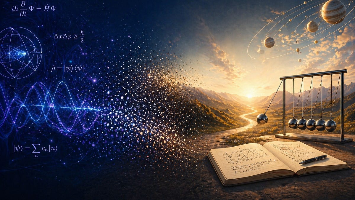
Quantum theory translates between waves and classical probabilities in a straightforward mechanism called decoherence. You can think of decoherence as when many, many waves interact with one another, their phase coherence (how their peaks and troughs line up) is destroyed. The result is that phase information becomes less and less important, and all that matters is the different probable outcomes.

This is how we go from Schrodinger’s cat to a dead or alive cat.

Decoherence is necessary for all objective interpretations of quantum mechanics, including the Many Worlds. Ultimately, decoherence is what “separates” the worlds from one another, since before that their phase coherences keep them locked together. Technically, the worlds aren’t separate after decoherence; either they are just phase incoherent, so they can no longer interact.

Decoherence, however, can only remove phase coherences. It cannot tell you what the actual outcome is going to be. In other words, it can tell you that the cat is alive or dead, but not which one it will be.

It is what happens after (or during) decoherence that tells us what quantum mechanics is actually doing.

While some believe we split into many universes, others believe that conscious observation somehow causes decoherence to transition to a single decohered state: alive or dead, up or down, true or false.

Those who believed in the observation-triggered collapse, however, have a problem. They can not explain precisely how or why this would happen.

Enter: objective collapse theory.

The goal of objective collapse theory is to explain this mechanism. Starting in 1986, a model was introduced by Ghirardi, Rimini, and Weber that showed how quantum theory could be modified so that, not only would decoherence happen over time, but the wavefunction itself would spontaneously, without even needing to be observed, collapse all on its own, like a house of cards in a gust of wind.

Their first model included these things called jump operators, which meant that collapse would happen very suddenly with these random, “localization” events called “hits”. (Localization is another word for wavefunction collapse, especially when it occurs for position.)

This means that at random times, according to a probability distribution, the wavefunction would just collapse, whether anyone was looking at it or not.

Later on, in 1990, GRW adapted their model to another kind of spontaneous collapse theory called Continuous Spontaneous Localization (CSL). In this case, the collapse didn’t happen suddenly and randomly but over time. So instead of the house of cards falling over from a sudden gust of wind, it fell down by a thousand little puffs of air.

Think for a moment how things might be different if either of these mechanisms proved true: we would finally know how classical physics emerges from quantum. Our need to find interpretations for that part, at least, would be at an end. Perhaps the wavefunction, or its field theoretic equivalent, really is the fundamental reality, but it is an unstable reality, whereas classical physics is its stable state.

I, for one, like objective collapse theories because they remove the hokiness of believing that conscious minds somehow create the universe with all its attendant philosophical difficulties. It also removes the existential discomfort that the Many Worlds interpretation causes many of us, believing that there are a multitude of copies of ourselves running around in parallel worlds.

Instead, there would be one world: this one, one past, one future, and one you. Unique.

What is happening at the quantum level, although it ultimately determines reality, has limits.

The downside to GRW and what is now called CSL is that both have to modify quantum mechanics by introducing randomness to force the wavefunction to collapse over time (either probabilistically from “hits” or continuously from noise).

This is a serious claim: Quantum mechanics as-is isn’t good enough.

I took this problem head-on in the last few months, although I got there by a circuitous route. My goal: show that quantum mechanics is good enough by itself to collapse the wavefunction.

For a long time, as I have frequently written about here, I have been looking for a theory that would explain quantum mechanics itself. I believed that a five-dimensional universe would, in fact, explain exactly where it comes from.

I became fixated on the idea that classical physics in compact, curled-up dimensions could lead to quantum theory.

And I failed. Instead of reproducing quantum mechanics, I derived an equation that would later prove to me that I had had it backwards the whole time. Quantum mechanics didn’t come from classical. It was the other way around.

In the process, I stumbled into a whole area of quantum physics that I had never encountered before, but which I eventually realized could explain the CSL model.

There is a subfield, going back at least to the 1960s when a lot of the best work on quantum mechanics and field theory was done, called open quantum systems. In physics, a closed system means that your model includes everything; nothing is getting in, and nothing is getting out. A system is open when your model does not include everything. This implies, of course, that the things getting in and getting out of your open system are models, but whatever is causing them to get in and out is not being modeled.

Take a model of a greenhouse as an example. You can model the conditions inside a greenhouse without modeling the nuclear fusion taking place in the sun, nor the ambient temperatures impinging on the exterior of the glass, nor the exterior air currents that may affect your ventilation. All these external influences can be abstracted away.

In other words, you don’t have to model the full water cycle to know that rivers flow downhill.

Quantum systems are no different. Why model 1000 molecules if you only care about one? Instead, abstract the 1000 molecules into some external force.

This is exactly how models of Brownian motion work, too. We don’t model all the individual molecules knocking a bit of pollen around in a petri dish. All we care about is how the collective energy of the molecules influences the pollen.

Albert Einstein explained this in one of his 1905 annus mirabilis papers. His main result in that paper (which is often forgotten as it appeared alongside relativity and the photoelectric effect) was something called a fluctuation-dissipation relation or theorem. Such theorems are essential to understand how macroscopic objects interact with lots and lots of randomly moving microscopic objects.

Random motion in macroscopic objects includes these two opposing forces: fluctuation, which is random noise traveling from the environment to the object, and dissipation, which is energy leaking from the object into the noisy environment. These two together determine the random motion of the object, ensuring that the object doesn’t continually gain energy and acceleration from noise, but also never stops from dissipation. Rather, the two balance each other out.

Open quantum systems likewise have noise and dissipation as their primary opposing elements, but calculating them is a lot more complicated.

This all started around 1963 when Richard Feynman and a student named Frank Vernon were working on a PhD in electrical engineering and physics. (He passed away in 2002 but is sometimes confused with a professor of the same name at UCSD.) Together, they used Feynman’s prior research into quantum theory to develop a theory of open quantum systems, where complicated quantum environments could be abstracted away into expressions for fluctuation and dissipation.

This was pretty monumental in itself, but nothing compared to what would become of it later.

There are two kinds of open systems: those that are in equilibrium with their environments and those that are not.

If a macroscopic object is in equilibrium with its environment, that means that where it ends up is pretty much the same as where it started, at least in terms of its probable location. If I have a piece of pollen in a petri dish, I can take a snapshot of where it is now and work either forward or backwards in time to determine where it is likely to be and where it is likely to have been. The probability for where it has been any time in the past, however, will match the probability for the future. That is what equilibrium means. Time doesn’t matter. Nothing is going anywhere in a definite sense.

The pollen isn’t expected to change because of what’s happening.

But if I replace the pollen with something fragile, a mini-house of cards, then I would expect at some point the house of cards would collapse. Since I don’t expect houses of cards to magically assemble themselves, if I work backwards in time, if I see a house of cards now in a noisy environment, I would expect that house of cards to still be there any time in the past. Once it has collapsed, however, I expect that it will remain collapsed forever.

This is an example of a non-equilibrium system. In fact, it is not only not in equilibrium, but it is also an irreversible process. The house of cards cannot reassemble itself.

In physics, equilibrium processes are comparatively easy to understand. There isn’t anything dynamic about them. It is all statistical. I did my PhD thesis on equilibrium statistics, and I can tell you that it is a lot easier to model something that doesn’t change over time than something that fundamentally does.

Perhaps the most confusing thing about modeling quantum systems is how they work in time. Open quantum systems do not evolve from one time to the next the way that classical systems or closed quantum systems do. They evolve along a contour that goes from the infinite past up to the point in time you care about and then back to the infinite past.

In other words, they evolve along an infinitely long, closed time-loop, which sounds like an interesting plot device for a science fiction novel, but is actually critical to understand how open quantum systems differ fundamentally from other kinds.

In open quantum systems, we don’t often work directly with the wavefunction but with an object constructed from wavefunctions called a density matrix.

A density matrix is like a probability distribution except that it includes all the phase information that quantum wavefunctions have as well as probabilities.

Because a density matrix is formed from two wavefunctions, the way you evolve the matrix as a whole forward in time is you actually evolve the left side of the matrix forward in time and the right side backward in time.

Yes, the density matrix lives on two time lines, a forward line and a backward line, straddling them like Colossus of Rhodes (which didn’t actually straddle the harbor, but that’s the expression).

In any closed quantum system, you can treat the timelines as separate entities, but in an open quantum system, you are getting rid of part of the matrix corresponding to your environment and only retaining the part you care about.

The forward side of the system and its backward side interact with the same environment. Because the environment is the same for the forward and backward sides, the timelines become stuck together so that the same environment interacts.

Feynman and Vernon dealt with this issue by making two copies of their system, a forward copy and a backward copy. They then enforced the copies to coincide with each other at the time they were interested in. This forced them to form a closed loop. The forward side comes from the infinite past up to the time of interest, and the backward side goes from that time of interest to the infinite past.

If this makes your head spin as it does mine, imagine the system as being like a time traveler in a universe where the rules of time travel are very strict. In order to retain their identity, a time traveler who travels forward in time must return to their exact place of origin in the past where they left. In other words, their path through time must form a closed loop. If their path does not follow this closed loop, then not only will the time traveler be split in two, but the universe will be split as well! The universe is analogous to the environment. If you want there to be only one universe, your time traveler has to return to the past.

Although Feynman and Vernon had laid the foundation, it took Soviet physicist Leonid Veniaminovich Keldysh to make the conceptual shift and build the house. All Feynman and Vernon had really done was explain how systems decohere when interacting with an environment. They had related this to noise and dissipation. Keldysh invented an entire nonequilibrium field theory. Instead of asking what happens to the density matrix, he asked what any physicist wants to know: what happens to the things we want to measure?

That then leads to what is called the Keldysh contour that the time traveler travels along.

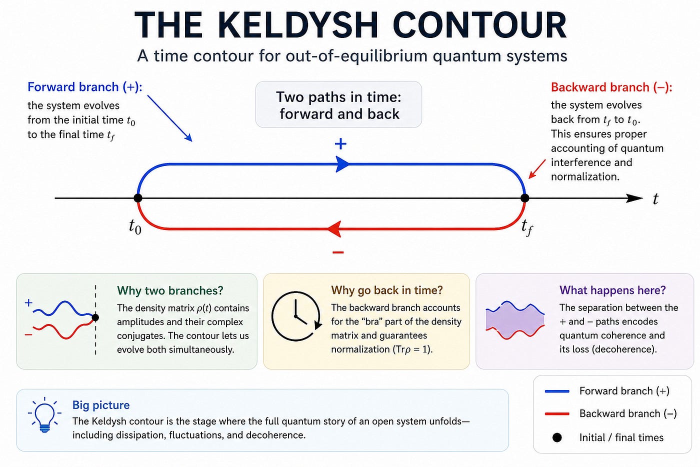
The Keldysh contour. Generated by ChatGPT.

If you were to look at the notation used in Keldysh theory, you would probably want to immediately turn back to your trusty quantum field theory textbook and never grace Keldysh’s door again, but if you do take the time, you will see that Keldysh does for quantum systems what Feynman had earlier done for ordinary quantum field theory. He made it understandable using diagrams.

I won’t go into his diagram method, but it is similar to Feynman’s in some ways.

Thanks to Keldysh’s work, I was able to start in earnest trying to understand how a quantum field could, thanks to a compact 5th dimension, collapse itself.

One of the things that happens when you have a tiny curled-up dimension is that you can take one field defined over all five dimensions with one particle mass and turn it easily into a lot of fields in four dimensions with a ladder of increasing particle masses. (This is called the Kaluza-Klein tower or KK tower.) If the original field interacts with itself, then all the resulting fields will interact with each other, and this is the first step in applying the Keldysh theory.

The lowest mass field in the KK tower has the same mass as the original field. I treated this as my system of interest. The rest of the tower I treated as my environment.

Thanks to the Keldysh contour theory, I was able to calculate the noise and dissipation for this kind of theory, and from that, pretty easily produce the same type of equation that is used in the CSL theory. So far, so good.

I then started to look at whether I would get good collapse from that.

I quickly found out that if the compact dimension was just a bunch of vacuum fields, meaning nothing in there, then collapse could not happen. The whole idea here, after all, is that the KK tower fields need to scramble the wavefunction in the observable field and cause decoherence. They have to force it to decohere. It turns out, however, that in a vacuum that can’t happen because the lightest KK tower will be too heavy (mass-wise), and if that one is too heavy, then the other tower fields are much too heavy.

If, on the other hand, the KK tower fields have some excitations in them, which could be primordial particles or something else, then those excitations can help scramble the wavefunction of the observable field. That’s interesting, of course, because that fits well with Kaluza-Klein dark matter theories, which propose that the universe is filled with such excitations.

It was in this moment that I realized that I had reproduced the CSL theory (under a whole heap of well-justified approximations, of course).

And that’s really all there is to it. My paper is now out on my website and has been submitted to a journal.

https://andersenuniverse.com/wp-content/uploads/2026/04/emergent_wavefunction_collapse_andersen_28apr2026.pdf

Ultimately, what it shows is that a compact 5th dimension can cause a quantum field theory to collapse its observable part while remaining an ordinary quantum field theory. No modifications to Schrodinger’s equation, no information destruction at collapse. It’s all emergent. The lost information just escapes into the compact dimension where it is irretrievable.

This has made me wonder if, philosophically, my chasing after a way to derive quantum mechanics from classical all these years wasn’t a fool’s errand, a kind of philosophical irritation with quantum theory that, I feel, I have resolved by showing that it is the other way around.

Originally published at https://timandersen.substack.com.