MATHEMATICS EXPLAINED

The Idea That Taught Mathematics To Move

How derivatives grew from tangents and motion into the language of gradients, optimization, and machine learning

A curve looks still on the page.

It may sit there as a black line on white paper, frozen between two axes, apparently doing nothing. But at every point, the curve carries a hidden instruction. It tells us whether it is rising or falling. It tells us how quickly it is changing. It tells us where it begins to flatten, where it bends more sharply, where it is about to turn.

The parabola y = x² looks still on the page, but every point carries local information about direction and rate of change.

The derivative is the mathematical device that reads this instruction.

This is why calculus feels different from much of the mathematics that comes before it. Arithmetic counts. Algebra rearranges. Geometry measures shape. Calculus begins to ask what happens when something changes. Not after a large step. Not between two distant positions. But here, at this point, under an almost invisible movement of the input.

That is a strange question.

If a car travels 100 kilometers in two hours, its average speed is 50 kilometers per hour. That is easy. But what is its speed at one exact instant? If the profit of a company depends on production, what is the effect of producing one more unit?

The derivative was invented for questions like these.

It began with curves and motion. It became a language for rates, sensitivities, approximations, and optimization. Today, the same old idea lives inside scientific computing, engineering design, economics, control systems, and machine learning.

Every time a model learns by following a gradient, it is using a descendant of the same idea that once helped mathematicians understand the slope of a curve.

When Mathematics Began To Chase Motion

The derivative did not appear fully formed in one moment.

Before Newton and Leibniz, mathematicians had already been moving toward it. They studied tangents to curves, areas under curves, maxima and minima, and the geometry of motion. Fermat had methods for finding extrema. Descartes and others had shown that curves could be treated algebraically. The ground was already prepared.

But in the seventeenth century, the problem became unavoidable.

Astronomy, mechanics, and geometry were all asking questions that ordinary algebra could not answer cleanly. Planets moved. Projectiles curved through space. Falling bodies accelerated. Curves needed tangents. Physical quantities changed continuously.

Mathematics needed a way to describe motion without breaking it into crude pieces.

Newton approached the problem through motion. He thought of quantities as flowing. A position changed with time. The rate of this flow was what he called a fluxion. His language was deeply connected to mechanics, to velocity, and to the physical world.

Leibniz approached the problem through differences. He introduced a symbolic notation based on small changes: dx and dy. The ratio dy/dx became one of the most successful pieces of notation ever invented. It did not only describe a calculation. It suggested a way of thinking. A tiny change in x produces a tiny change in y, and their ratio tells us how y responds to x.

Isaac Newton on the left, whose fluxions grew from motion, and Gottfried Wilhelm Leibniz on the right, whose differential notation shaped the way calculus is still written. Images: Godfrey Kneller, Portrait of Isaac Newton (1689); Christoph Bernhard Francke, Portrait of Gottfried Wilhelm Leibniz (c. 1695), via Wikimedia Commons, public domain.

Newton and Leibniz later became attached to one of the most famous priority disputes in the history of mathematics. But the derivative itself is larger than that dispute. The deeper point is that mathematics had found a way to describe change locally.

This was the decisive shift. Instead of asking only where something is, calculus asked how it is changing there.

The Problem With The Slope Of A Curve

The slope of a straight line is simple.

Take two points. Measure the vertical change. Measure the horizontal change. Divide one by the other.

The line has the same slope everywhere. It does not matter where the two points are chosen. The line is loyal to one direction.

A curve is different.

A curve does not have one slope. It bends. It may rise steeply, then flatten, then fall. On one part of the curve, the slope may be positive. Somewhere else, it may be zero. Later, it may become negative. There is no single number that describes the whole curve.

So the real question becomes more delicate. What is the slope of a curve at one point?

A tangent line touches a curve at a single point, turning the local behavior of the curve into the slope of a straight line. Image: Tangent to a curve.svg, via Wikimedia Commons, public domain.

To compute a slope, we need two points. But the question asks for the slope at one point. One point alone does not give a rise and a run. It gives a location, not a direction.

The solution is one of the great ideas in mathematics.

Start with two points on the curve. Compute the average rate of change between them. Then move the second point closer and closer to the first. The secant line becomes less like a broad measurement across the curve and more like a local measurement near one point.

In the limit, if the process behaves well, the secant line becomes the tangent line.

That limiting slope is the derivative.

For a function f(x), the derivative is written as

This formula looks small, but we should see it work at least once.

Take the simplest curved function:

Then the average rate of change from x to x + h is

So we get

Expanding the square gives

The x² terms cancel and h can be factored out:

So the average rate of change becomes

This is still a slope between two nearby points. But now we let the second point move closer to the first. In other words, h goes to zero.

What remains is

So the derivative of x² is 2x.

That means the slope is not the same everywhere. At x = 1, the slope is 2. At x = 3, the slope is 6.

The same idea applies to any smooth curve, not only to x². A more complicated curve simply makes the changing slope easier to see: as the point slides along the curve, the tangent line turns with it.

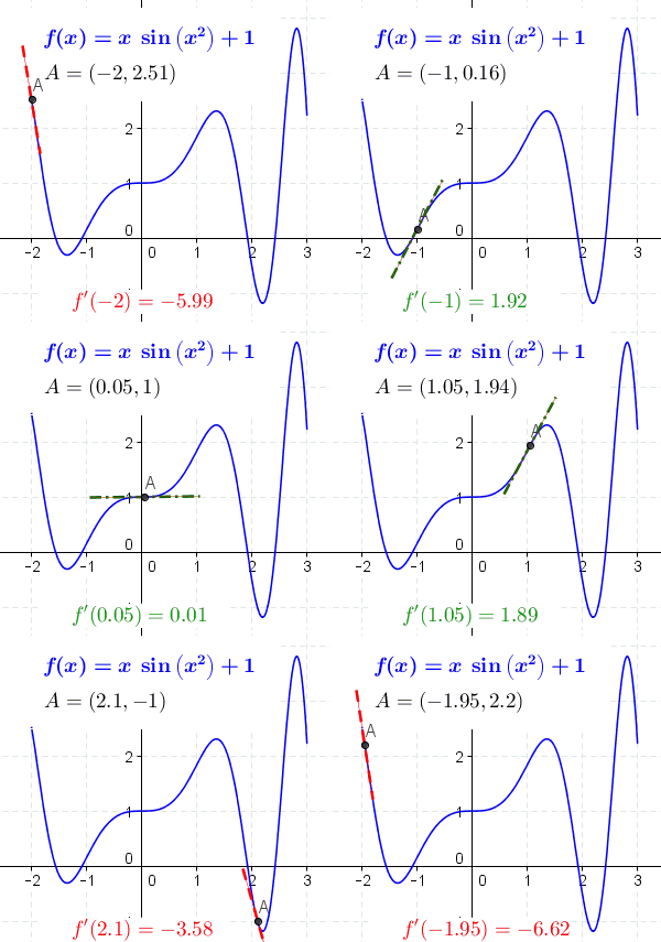
After the simple parabola example, a more complicated curve shows the same idea in motion: as the marked point travels, the tangent line turns, and the derivative records the local slope at that position. Image: Dino and Lfahlberg, via Wikimedia Commons, CC BY-SA 3.0.

This is the meaning of the derivative.

It takes an ordinary average change over a finite interval and compresses the interval until it almost disappears. What remains is not an average over a distance, but an instantaneous rate of change.

The Local Line Hidden Inside A Curve

There is another way to understand the derivative.

Near any sufficiently smooth point, a curve behaves almost like a line.

Not exactly. If we zoom out, the curve may bend dramatically. But if we zoom in enough near one point, the curve begins to look straight. The derivative gives the slope of this local line.

ANIMATION: The parabola f(x) = x² is magnified around a point. At smaller scales, the curve becomes almost indistinguishable from its tangent line, whose slope is given by the derivative f’(x) = 2x.

This is why the tangent line is not just a drawing on a graph. It is a local approximation. It says: near this point, the function behaves approximately like this straight line. That is one of the most powerful ideas in applied mathematics.

In engineering, we often do not understand a complicated system all at once. We understand it locally. We linearize. We perturb. We ask what happens when a parameter changes slightly. We study sensitivities. We replace a nonlinear problem, temporarily and carefully, by something linear enough to handle.

The derivative is the basic mathematical object behind this habit.

The derivative gives us local information. It does not tell us everything. It does not reveal the whole curve. It does not automatically solve the whole problem. But it tells us what the function is doing nearby. In many large problems, that is already a lot.

The Derivative Has Many Faces

The derivative is often introduced as the slope of a tangent line. That is correct, but it is only one face of the idea.

In mechanics, the derivative of position with respect to time is velocity. The derivative of velocity with respect to time is acceleration. This is not a metaphor. It is exactly the same mathematical operation, applied to motion.

If s(t) is position, then s'(t) gives velocity. If v(t) is velocity, then v'(t) gives acceleration. A moving object does not merely have a position. It has a tendency. It is going somewhere. The derivative captures that tendency.

In economics, the derivative appears as a marginal quantity. Marginal cost asks how total cost changes when production increases slightly. Marginal revenue asks how revenue changes when one more unit is sold. These are derivative ideas, even when the real world is measured in discrete units.

In biology, derivatives describe growth rates. In chemistry, they appear in reaction rates. In control systems, they describe how signals change. In optimization, they tell us how to improve a quantity. In machine learning, they tell a model how to adjust its parameters.

The notation changes. The story does not.

Rules That Made Change Calculable

The limit definition explains what a derivative is. But if every derivative had to be computed from the limit definition, calculus would be painfully slow.

The power of calculus came from rules.

The derivative of a constant is zero. A constant does not change, so its rate of change is zero. The derivative of x is one. The derivative of xⁿ is

This immediately turns a polynomial into something easier to read. For example, if

then

The original expression describes the quantity. The derivative describes how that quantity changes.

This is why the rules mattered so much. A complicated expression could be broken into smaller pieces. Instead of returning to the limit every time, one could use a symbolic machinery. Algebra and calculus became partners.

Among all the rules of differentiation, one rule became especially powerful. The chain rule.

The Rule That Lets Change Flow Through A System

Many quantities do not depend directly on one variable. They depend on something that depends on something else.

For example, take the function

This is not just one operation. It is a function inside another function. First, x is turned into an intermediate quantity:

Then that intermediate quantity is cubed:

So the original expression can be understood as a chain:

Now the question becomes: what is the total effect on y?

The change must pass through two layers. First, x changes u. Then u changes y. In Leibniz’s notation, the chain rule says:

It is tempting to say that the du terms cancel. That is not the full rigorous story, but it captures the intuition very well. A small change in x first produces a small change in u. That small change in u then produces a small change in y. The total effect is obtained by multiplying the two local rates.

In our example,

so

Also,

so

Multiplying the two local rates gives

Finally, we replace u by x² + 1:

The same rule is often written in function notation. If

then

The formula is not just a symbolic trick. It says that influence travels through the inner quantity first, and then through the outer one. A small change at the beginning is transformed as it moves through the chain.

This is one of those formulas that looks like a school exercise until we realize how much of the modern world is built from nested dependencies.

The chain rule tells us how influence propagates through a sequence of dependencies.

This is why the rule later became so important in modern computation. A neural network is also a composition of functions: one layer transforms the data, the next layer transforms the result, and the process continues. The full machine-learning story comes later, but the mathematical skeleton is already visible here.

A rule that began as a way to differentiate composite functions became a way to track influence through many layers.

From One Direction To Many

The derivative is easiest to understand when there is one input variable.

A function f(x) takes one number and returns one number. The derivative tells us how the output changes when x changes. There is only one direction to move: left or right along the x-axis.

But most real problems are not one-dimensional.

A design problem may have many variables. A financial model may depend on many market variables. A climate model may depend on enormous fields of interacting quantities. A machine-learning model may contain millions or billions of weights.

In such cases, there is no single derivative. There are partial derivatives.

A partial derivative asks how the function changes when one variable changes while the others are held fixed. This assumption is not always physically simple, but mathematically it gives us a way to separate the local effects of different variables.

For a function f(x, y), we can ask how f changes with respect to x. We can also ask how f changes with respect to y.

These are written as

and

The symbol changes from d to ∂ because we are no longer dealing with one independent direction. We are measuring change along one coordinate direction while the other variables are treated as fixed.

This is the beginning of multivariable calculus.

In one variable, local behavior is captured by a tangent line. In two variables, the analogous object is a tangent plane. A smooth surface may curve in many directions, but near one sufficiently regular point, it can still be approximated by a plane. The idea is the same: calculus replaces a small piece of something curved with something linear enough to understand.

A tangent plane touches a sphere at one point, showing the multivariable version of the tangent idea: near a smooth point, a curved surface can be approximated by a plane. Image: Alexwright at English Wikipedia, Image Tangent-plane.svg, via Wikimedia Commons, public domain.

And once we have many partial derivatives, we can collect them into one object. The gradient.

The Gradient Is A Compass

The gradient of a function is a vector made from its partial derivatives.

For a function f(x₁, x₂, ..., xₙ), the gradient is

This notation may look more advanced, but the idea is direct.

Each partial derivative tells us how the function changes in one coordinate direction. The gradient gathers all these local sensitivities into one vector.

Then comes the geometric fact that makes the gradient so useful: The gradient points in the direction of steepest increase.

The surface of the function f(x,y) = -(cos²x + cos²y)², with its gradient shown as a projected vector field on the bottom plane. Image: MartinThoma, via Wikimedia Commons, CC0 1.0 Universal Public Domain Dedication.

Imagine standing on a landscape. Your height is the value of a function. The ground rises in some directions and falls in others. The gradient points uphill as steeply as possible. If you want to climb fastest, follow the gradient. If you want to descend fastest, move in the opposite direction.

This picture is simple, but it scales surprisingly far.

In two dimensions, we can imagine a landscape. In three dimensions, perhaps we can still visualize something. In a million dimensions, we cannot see the landscape at all. But the mathematics still works. The gradient still gives a local direction.

This is the extraordinary thing. A neural network with millions of parameters has a loss function defined over a space we cannot visualize. There is no drawing of this landscape that our intuition can fully grasp. Yet the gradient still provides a direction in that high-dimensional space.

It says: locally, this is the way the loss increases fastest. So we usually go the other way.

Optimization Is Calculus With A Goal

Optimization is the search for the best choice.

The lightest structure that satisfies safety constraints. The least expensive route. The most efficient shape. The best-fit parameters of a model. The smallest prediction error. The maximum profit.

These problems may look different, but mathematically they often have the same structure. There is an objective function, and we want to make it as small or as large as possible.

Derivatives enter because maxima and minima are connected to flatness.

In one dimension, a smooth function often reaches a local maximum or minimum where the derivative is zero. At such a point, the function is no longer increasing or decreasing to first order. The tangent line is horizontal.

Local maxima and minima often occur where the curve becomes flat. At these points, the tangent line is horizontal and the first derivative is zero.

This is not a guarantee of a true optimum. A derivative equal to zero can also indicate a saddle-like behavior in higher dimensions, or a point where the function merely pauses before continuing. But it gives candidates. It tells us where something interesting may happen.

In many dimensions, the equivalent condition is that the gradient vanishes.

At such a point, there is no immediate first-order direction of increase or decrease. The function is locally flat in the sense measured by the gradient.

For small problems, one may try to solve these equations directly. But modern problems are often too large for that. Instead, optimization usually becomes iterative.

We do not jump to the answer. We move. We evaluate the function. We compute or estimate the gradient. We take a step. Then we do it again.

The simplest version is gradient descent. Move in the direction opposite to the gradient. The rule is often written as

The parameter α is the step size. If it is too small, progress is slow. If it is too large, the method may overshoot, oscillate, or diverge. The derivative gives a direction, but the algorithm still has to decide how far to trust it.

This is a useful reminder. The derivative does not give the whole answer at once. It gives a local instruction. Optimization turns many local instructions into a path.

Gradient descent turns local derivative information into a path. Starting from an initial point, each step moves in a direction that reduces the objective function, gradually approaching a minimum. Image: Zerodamage, Gradient descent.svg, via Wikimedia Commons, public domain.

The Second Derivative And The Shape Of Change

The first derivative tells us how a quantity changes. The second derivative tells us how the change itself changes.

In motion, the first derivative of position is velocity, and the second derivative is acceleration. If velocity is changing, acceleration measures that change.

In geometry, the first derivative describes slope. The second derivative describes concavity. It tells us whether the curve bends upward or downward.

In optimization, the second derivative helps us understand the shape of the objective function near a point. A point with zero first derivative may be a minimum, a maximum, or neither. The second derivative provides curvature information.

For a one-dimensional function, if the first derivative is zero and the second derivative is positive, the function locally bends upward. This suggests a local minimum. If the second derivative is negative, it bends downward. This suggests a local maximum. If the second derivative is zero, the test may tell us nothing.

In many dimensions, second derivative information becomes the Hessian matrix. Instead of a single second derivative, we now have a whole array of second partial derivatives:

This matrix records local curvature in many directions at once. The diagonal entries show how the function bends along each variable individually. The off-diagonal entries show how the variables interact.

In optimization, Newton’s method uses this second-derivative information directly. Gradient descent follows the slope; Newton’s method also asks how that slope is changing.

The gradient says which way is uphill. The Hessian says how the landscape bends.

This matters in real problems because not all landscapes are friendly. Some are steep in one direction and flat in another. Some contain narrow valleys. Some have saddle points. Some are noisy. Some are not smooth at all.

The gradient starts the search. The Hessian tells the search what kind of terrain it is entering.

The Derivative In Engineering Thinking

For an engineer, the derivative is not only a mathematical operation. It is a way of thinking about systems.

A structure responds to loads. But the response depends on stiffness, geometry, supports, mass distribution, damping, material nonlinearity, boundary assumptions, and modelling choices. We rarely know everything with absolute certainty. We often ask how sensitive the result is to a parameter.

If a small change in a parameter produces a large change in the response, the system is sensitive. If the response barely changes, the parameter may be less critical for that quantity of interest.

This is derivative thinking.

In structural optimization, the objective may be weight, cost, compliance, embodied carbon, or some measure of performance. The constraints may include stress limits, displacement limits, buckling conditions, natural frequencies, constructability, or code requirements. A design variable may control a section size, a topology parameter, a shape coordinate, or a material distribution.

The derivative of the objective or constraint with respect to the design variables tells us how the design wants to change.

Of course, engineering problems are rarely as clean as textbook functions. Models may be nonlinear. Constraints may be active or inactive. Design spaces may be discrete. Numerical approximations may introduce noise. A derivative may be exact, approximate, or unavailable.

Still, the conceptual role remains clear. The derivative is a local sensitivity measure. It tells us how strongly a model output reacts when assumptions, parameters, or loads are perturbed.

That is why derivatives appear in finite element analysis, inverse problems, parameter identification, uncertainty quantification, reliability analysis, topology optimization, and control.

Why Machine Learning Needed Calculus

Machine learning is sometimes presented as something new enough to have escaped older mathematics. It has not.

Modern machine learning uses new data, new computational power, and new architectures. But the basic training mechanism of many models is deeply connected to calculus.

A model has parameters. These may be regression coefficients, tree-splitting parameters, weights in a neural network, or other adjustable quantities depending on the method. For neural networks, the number of weights can be enormous.

Diagram of a feedforward neural network, showing input nodes, hidden layers, weights, biases, activations, and a single output. Image: QuantuMechaniX8, via Wikimedia Commons, CC0 1.0 Universal Public Domain Dedication.

The model makes a prediction. The prediction is compared with the desired output. The difference is measured by a loss function.

Training means changing the parameters so that the loss decreases.

This is exactly where derivatives enter. For each parameter, the algorithm needs a sensitivity: whether increasing that parameter would raise or lower the loss, and by how much.

That sensitivity is a partial derivative. For all parameters together, the partial derivatives form the gradient of the loss function.

Then the learning algorithm updates the parameters, usually by moving them in a direction that reduces the loss. This is why gradient-based optimization became so central to deep learning.

The chain rule enters because a deep neural network is not a single simple formula. It is a layered composition. A weight in an early layer affects an activation. That activation affects the next layer. That layer affects another layer. Eventually, all of this affects the final prediction and the loss.

The effect of one weight on the loss is distributed through the chain.

Backpropagation computes these effects efficiently.

Without derivatives, training large differentiable models would be almost blind. The algorithm could try random changes and keep the ones that help, but that would be hopelessly inefficient in high-dimensional spaces. The gradient gives direction. It does not make learning easy, but it makes learning possible at scale.

This is why the derivative, invented in the age of falling bodies and tangents, now appears inside systems that translate text, generate images, recommend videos, recognize speech, and optimize engineering designs.

The setting changed. The local calculation did not.

What The Derivative Cannot Do Alone

The derivative is powerful, but it is not magic. It is local. This is both its strength and its limitation.

A derivative tells us what happens near a point. It does not automatically tell us what happens far away. A function may descend locally and still lead us to a poor minimum. A zero derivative may suggest a candidate optimum, but it does not prove that the point is globally best. A gradient may point downhill, but the landscape may contain traps, plateaus, sharp valleys, or saddle points.

There is another assumption hidden in the background.

The derivative requires smoothness, or at least some form of differentiability. Many real systems contain discontinuities, thresholds, impacts, contact, cracking, yielding, switching behavior, or discrete decisions. In such cases, classical derivatives may fail or may need to be replaced by generalized ideas.

Numerical derivatives also carry practical difficulties. A finite difference may depend on the chosen step size. A step that is too large misses local behavior. A step that is too small may suffer from round-off error. Automatic differentiation avoids many of these problems for computational graphs, but it still differentiates the model we wrote, not necessarily the physical reality we hoped to represent.

The assumptions decide how far the local calculation can be trusted.

The Old Idea Inside Modern Machines

The derivative began with a geometric question that seems almost innocent: how can a curve have a slope at one point?

From that question came a language of instantaneous change. It explained velocity and acceleration. It turned tangents into calculations. It made maxima and minima searchable.

Then the idea expanded. One derivative became many partial derivatives. Many partial derivatives became a gradient. The gradient became a compass in high-dimensional spaces. Optimization turned that compass into a path. Machine learning used that path to train models with millions or billions of parameters.

Calculus did not predict artificial intelligence. The story is more interesting than that.

A mathematical idea invented for curves and motion turned out to be the right language for systems where small changes matter.

The derivative is how mathematics reads local direction. It does not see the whole journey. It does not know the final destination.

And sometimes, one local direction after another is enough to move through a world too complicated to understand all at once.

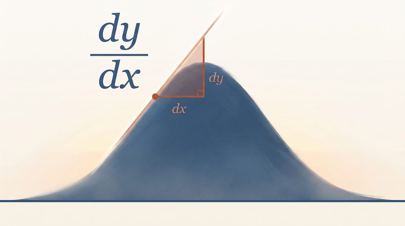
Cover image: A tangent line and the ratio dy/dx show how the derivative reads the local slope of a curve. Generated with AI tools for this article.