When Diffusion Models Learn the Wrong Physics

A deep dive into adaptive Fokker-Planck regularization and physics-informed distillation for molecular dynamics

image created by nano-banana

There’s something unsettling about training a diffusion model to generate molecular configurations. You can watch the loss curves go down. You can sample from the model and recover beautiful equilibrium distributions that match your training data almost perfectly. But then you ask the model to predict forces, and it gives you something physically meaningless.

This is the uncomfortable reality of applying score-based diffusion models to molecular dynamics. The models learn to denoise. They learn to match distributions. But somewhere in that training process, they miss something fundamental about the physics they’re supposed to represent.

The problem isn’t obvious at first. When you use these models for standard iid sampling (just generating configurations from noise), everything looks fine. The configurations are chemically reasonable. The energy landscapes seem plausible. It’s only when you try to run actual molecular dynamics, when you try to propagate trajectories forward in time using the learned force fields, that things fall apart.

The Score Function and the Fokker-Planck Equation

Let me explain what’s happening mathematically. Score-based diffusion models learn a time-dependent vector field sθ(x, t) that approximates the gradient of the log probability density:

For molecular systems at equilibrium, configurations follow the Boltzmann distribution. As diffusion time approaches zero, the score should converge to:

where U(x) is the potential energy. This is beautiful. The score at t=0 directly gives you the force field up to a temperature factor.

But here’s where things get subtle. The time evolution of the probability density pt(x) under the forward diffusion process must satisfy the Fokker-Planck equation:

where FFP is a nonlinear operator involving divergence and squared-gradient terms. When this equation is violated, your learned score function and its associated density evolve inconsistently over diffusion time. The model has learned endpoints (the data distribution at t=0) while getting the path completely wrong.

Standard denoising score matching optimizes for matching the data distribution through sampling. It doesn’t directly enforce that the learned score satisfies the Fokker-Planck equation. As a result, you can end up with models that generate perfect samples through reverse-time integration, but whose score at t=0 gives forces that violate basic physics. There might be spurious energy minima. The forces might not be conservative. The equilibrium distribution implied by these forces might differ from the one you trained on.Figure 1 from Plainer et al. illustrates this perfectly. A 2D toy example with two modes shows that standard diffusion training can learn the correct distribution for sampling while simultaneously learning an incorrect third mode. The diffusion sampling process never goes there, so samples look fine. But evaluate the score at t=0 to define forces, and molecular dynamics will happily explore that nonphysical region.

adopted from: Plainer, Michael, et al. (2025)

Enforcing Physical Consistency Is Expensive

So we need to enforce Fokker-Planck consistency. The approach is conceptually straightforward. Define a residual that measures how badly the learned score violates the equation:

Then add this as a regularization term:

where Ldsm is the standard denoising score matching loss. Computing this residual requires evaluating time derivatives and divergence operators, which involve expensive second-order operations.

Recent work uses a weak formulation that avoids explicit second derivatives by introducing small Gaussian perturbations:

where v ~ N(0, σ²I). The FP loss becomes:

And the time derivative is approximated using finite differences:

This helps, but computing FP residuals everywhere remains expensive. You need multiple score evaluations per sample (for the perturbations), finite difference stencils for time derivatives, and careful handling of the divergence terms. For large molecular systems with thousands of atoms, this computational overhead becomes prohibitive. And even after paying this cost during training, you’re left with a large energy network that’s expensive to evaluate at inference time.

Adaptive Fokker-Planck Regularization

The key insight is that we don’t need to enforce physics everywhere. Fokker-Planck violations matter when they affect force accuracy in regions that actually influence molecular dynamics trajectories. But not all violations are equally harmful.

Consider where forces actually get used. During MD simulation, you evaluate the score at small diffusion times (near t=0) on configurations near the equilibrium distribution. Violations far from equilibrium or at large diffusion times don’t directly impact your forces. Computing expensive FP residuals there wastes resources.

So we introduce a gating mechanism. Before computing the expensive FP residual, we check diagnostic signals that are cheap to evaluate. The drift-diffusion ratio tells us whether we’re in a regime where physics matters:

where β(t) is the diffusion rate. Large DDR values indicate regions where diffusion dominates, which correlates with physical inconsistency. We also consider the signal-to-noise ratio:

These combine into a smooth gating score:

where σ(·) is the sigmoid function. Parameters k and SNRmin are thresholds, γ controls transition sharpness, and tscale provides smooth decay with diffusion time. The gate makes a hard execution decision. We compute FP residuals only for samples where the gate indicates potential physical inconsistency.

This dramatically reduces computational overhead. Instead of computing expensive residuals on every training sample, we selectively apply regularization where it matters. The training signal concentrates on regimes that determine force accuracy while staying silent elsewhere.

Energy-Based Parameterization

To guarantee conservative forces, we parameterize the model through a scalar energy function:

This ensures learned forces are conservative by construction. The score is just the negative energy gradient, so path independence is automatic. This matters for physical interpretability and guarantees that force fields derived from the model satisfy basic thermodynamic requirements.

Algorithm 1: Teacher Training with Adaptive FP Regularization

The complete training procedure looks like this:

The key difference from standard diffusion training is the gated FP regularization. We only compute the expensive residual when the gate indicates we’re in a regime where physical consistency matters.

Physics-Informed Distillation

Even after selective regularization gives us a physically consistent model, it’s still too expensive for long MD trajectories. Each force evaluation requires computing the energy and backpropagating through a deep network. We need to compress the teacher into a smaller student while preserving both equilibrium statistics and force accuracy.

Force (Score) Distillation

The primary objective forces the student score to match the teacher:

where st and ss are teacher and student scores. Since physical forces are proportional to the score in the low-noise limit, this directly transfers force information.

Selective FP Regularization on Student

To maintain physical consistency in the distilled model, we apply the same gated FP regularization to the student during training. This ensures the student inherits the teacher’s physical constraints.

Trajectory-Level Distillation

Matching forces pointwise doesn’t guarantee stable dynamics. Small errors accumulate over time integration. To capture dynamical stability, we compare short Langevin trajectories:

A trajectory matching loss is defined as:

This trajectory loss captures somethin

g essential that pointwise matching misses. When you propagate both models forward for 10–20 timesteps, differences compound. By minimizing trajectory deviation, we encourage the student to reproduce stable long-time behavior rather than just instantaneous predictions.

The complete distillation objective combines all three:

Algorithm 2: Physics-Informed Distillation

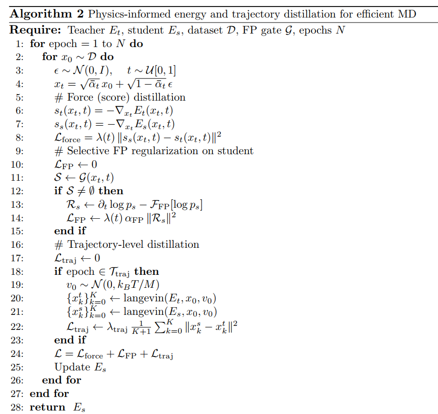
Teacher trajectories can be precomputed and cached to reduce cost. Trajectory loss is applied periodically rather than every iteration to balance computational expense with dynamical supervision.

Testing on Müller-Brown: Experimental Setup

The Müller-Brown potential is a classic 2D toy system with three metastable wells. It’s simple enough to visualize but rich enough to test sampling and dynamics. I generated a training dataset by running Langevin dynamics for 5.5 million steps, saving every 50th configuration to create 100k samples.

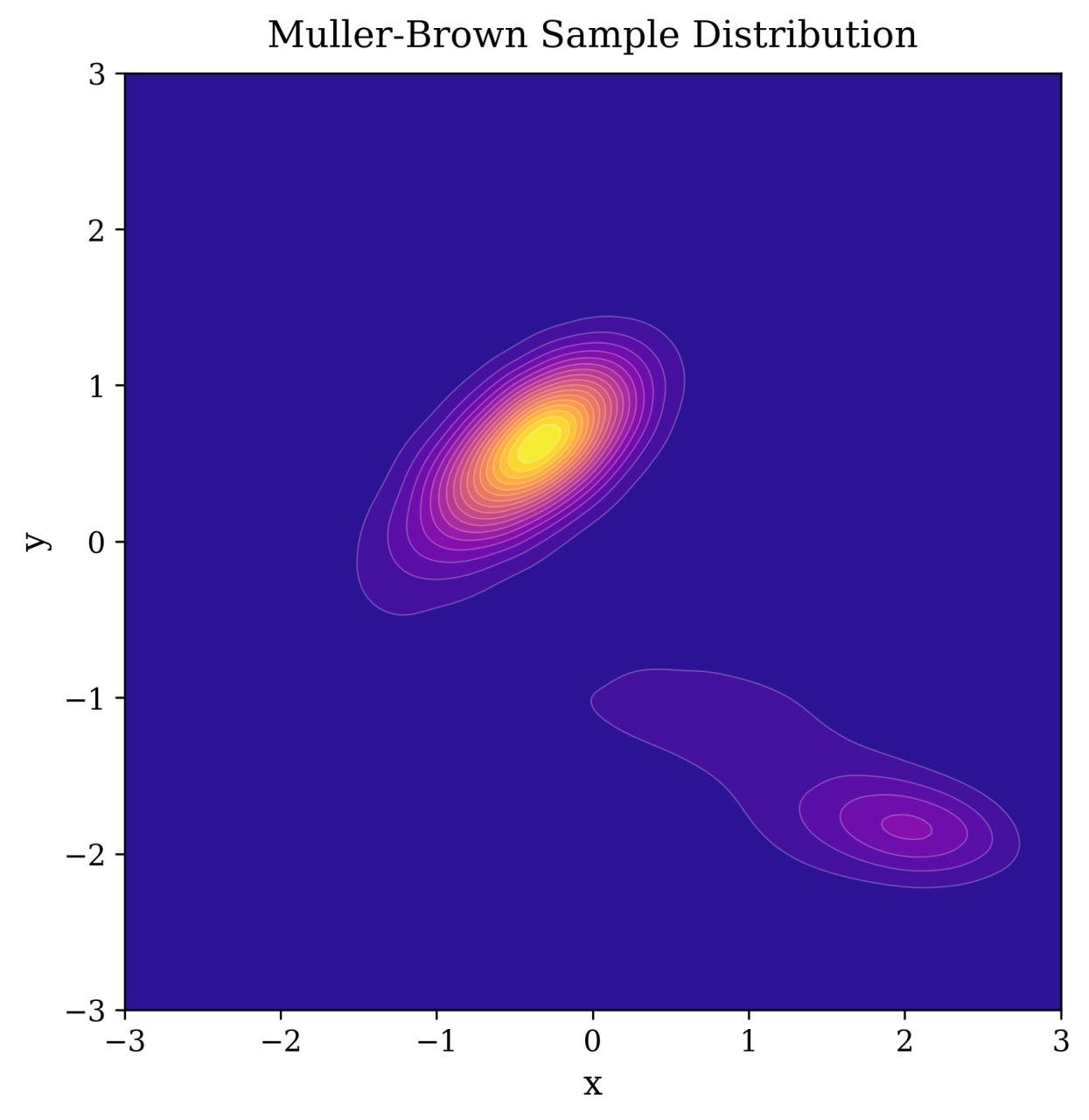
100k 2D points generated with Müller-Brown dynamics, showing three modes with different probabilities.

Global Hyperparameters

First, the global settings used throughout:

# ==== Global ====
DEVICE = 'cuda'

# ==== Langevin simulation ====
DT = 0.005; MASS = 0.5; GAMMA = 1.0
BURN_IN_RATIO = 0.5; KBT = 23.0

# ==== Diffusion network ====
INPUT_DIM = 2; HIDDEN_DIM = 128
TIME_EMBED_DIM = 128; NUM_BLOCKS = 3
ACTIVATION = 'silu'

# ==== Data ====
BATCH_SIZE = 128

# ==== Training ====
EPOCHS = 180; LR = 5e-5
GRAD_ACC = 2; WARMUP_STEPS = 10000

EPS_TIME = 1e-5  # time lower bound for stability

Dataset Generation

Creating the Müller-Brown dataset took about 6 hours on an i5–9300HF with GTX 1650:

# ~6h on i5-9300HF + GTX 1650 (4GB)
# set force_regenerate=True to create new data

dataset, potential = generate_muller_brown_data(
    n_samples=100000, dt=DT, mass=MASS,
    save_every=50, kbt=KBT, log_freq=500000,
    device=DEVICE, burn_in=500000,
    save_data=True, save_dir='./mb_data',
    filename='muller_brown_100k.pt',
    force_regenerate=False
)

Training Setup

I trained two models with identical architectures. One uses standard denoising without FP regularization. The other applies adaptive FP regularization through the gating mechanism.

dataloader = DataLoader(
    dataset, batch_size=BATCH_SIZE,
    shuffle=True, num_workers=1,
    drop_last=True
)

vs  = LinearVS(beta_min=0.1, beta_max=20.0)   # linear beta schedule
fwd = ForwardVP(vs)                           # VP-SDE forward diffusion

# Small diffusion network
fp_net = MullerBrownNet(
    input_dim=INPUT_DIM,
    time_embed_dim=TIME_EMBED_DIM,
    hidden_dim=HIDDEN_DIM,
    num_blocks=NUM_BLOCKS,
    activation=ACTIVATION
)

optim = torch.optim.Adam(
    [p for p in fp_net.parameters()], lr=LR
)

fp_trainer = MBTrainer(
    mb_net=fp_net, fwd=fwd,
    data_loader=dataloader, optim=optim,
    fp_gate=fp_gate,
    fp_loss=mb_fokker_planck_loss,
    noise_fn=noise_from_energy,
    fp_resid=mb_heavy_fp_residual,
    epochs=EPOCHS,
    device=torch.device(DEVICE),
    grad_acc=GRAD_ACC,
    checkpoint=10, log_freq=10,
    store_path="./fp_train",
    warmup_steps=WARMUP_STEPS,
    fp_alpha=5e-3,
    eps_time=EPS_TIME,
    gate_params={
        "k":1.0, "snr_min":0.5,
        "t_scale":0.1, "sharpness":8.0,
        "eps":0.01
    }
)

fp_losses = fp_trainer()

To disable FP regularization, set t_scale to zero in gate_params. This makes the gate always return false, so no FP residuals are computed.

Sampling

After training, we generate samples using both iid sampling and Langevin dynamics:

rev = ReverseVP(vs)

fp_sampler = MBSampler(
    model=fp_net, rev=rev,
    dataset_mean=dataset.mean,
    dataset_std=dataset.std,
    eps_time=EPS_TIME,
    store_path="./fp_samples",
    kbt=KBT
)

iid_samples = fp_sampler.iid_sampler(
    n_samples=50000,
    device=DEVICE,
    store_trajectory=False,
    return_original_space=False
)

lan_samples = fp_sampler.langevin_simulator(
    n_parallel=100, n_steps=30000,
    dt=DT, mass=MASS, gamma=GAMMA,
    device=DEVICE,
    save_every=100,
    burn_in_ratio=BURN_IN_RATIO,
    return_original_space=False
)

Figure 3 compares samples from both models. The top row shows results without FP regularization, bottom row with it. Each row displays true data, iid samples, and Langevin trajectories.

Comparison of samples from models with and without FP regularization. Top row: no FP-reg. Bottom row: with FP-reg. Columns: true data distribution, iid samples, Langevin dynamics sampling.

For this simple 2D system, differences are subtle. Both models produce reasonable samples. The Müller-Brown potential is forgiving enough that even models with some physical inconsistencies generate acceptable dynamics. This is expected. The real test comes in higher-dimensional systems where small inconsistencies compound. The experiment serves as proof of concept: the machinery works, gating reduces cost without breaking training, and models generate physically plausible samples.

Knowledge Distillation

With a trained teacher model, we can distill it into a smaller student. The teacher predicts how configurations evolve, giving us reference trajectories efficiently. During distillation, the student learns to reproduce teacher behavior while minimizing force loss, FP regularization, and trajectory loss.

Distillation Setup

# distilled (student) model
student_net = MullerBrownNet(
    input_dim = 2,
    time_embed_dim = 64,
    hidden_dim = 64,
    num_blocks = 2,
    activation ='silu'
)

print(
"Number of original (teacher) model's parameters: ",/
 sum(p.numel() for p in fp_net.parameters())
) 
print(
"Number of distilled (student) model's parameters: ",/
 sum(p.numel() for p in student_net.parameters())
)
# output:
# Number of original (teacher) model's parameters:  134529
# Number of distilled (student) model's parameters:  25921

That’s roughly 5x compression. The student has half the hidden dimension and one fewer block, dramatically reducing model size and inference cost.

# distillation optimizer which optimizes only student parameters
dist_optim = torch.optim.Adam(
[p for p in student_net.parameters()], lr=1e-5
)

dist_trainer = MBDistillationTrainer(
    t_net = fp_net,
    s_net = student_net,
    fwd = fwd,
    data_loader = dataloader,
    optim = dist_optim,
    fp_gate = fp_gate,
    fp_loss = mb_fokker_planck_loss,
    dist_loss = mb_distillation_loss,
    score_fn = score_from_energy,
    fp_res = mb_heavy_fp_residual,
    epochs = 150,
    device = DEVICE,
    grad_acc = GRAD_ACC,
    checkpoint = 10,
    log_freq = 10,
    store_path = "./mb_dist_train",
    warmup_steps = 10000,
    fp_alpha = 5e-4,
    gate_params = {
            "k": 1.2, "snr_min": 0.5, "t_scale": 0.1,
            "sharpness": 5.0, "eps": 0.1
        },
    traj_freq = 10,
    eps_time = 1e-5,
    compute_trajectory_loss = False
)
dist_losses = dist_trainer()

The compute_trajectory_loss flag controls whether to include trajectory-level supervision. For efficiency, you’d typically precompute teacher trajectories offline and load them during distillation. Setting traj_freq=10 means trajectory loss is evaluated every 10 epochs rather than every iteration.

Distillation Results

After distillation completes, we compare samples from teacher and student models. Figure 4 shows the comparison.

Comparison of sampling quality between teacher and student models. Top row shows teacher samples (true data, iid samples, Langevin trajectories). Bottom row shows student samples in same format. Both models reproduce the three-mode structure with similar statistics.

The distilled student produces samples that closely match both teacher and true data. Looking at iid samples and Langevin trajectories, you see the same three-mode structure with similar relative populations. The compression succeeded in transferring essential physics from teacher to student while dramatically reducing model size.

But keep in mind this is a toy dataset. The real question is whether this pipeline scales to realistic molecular systems with thousands of atoms and complex energy landscapes. That requires computational resources beyond what’s accessible for proof-of-concept work. The Müller-Brown experiments demonstrate the framework functions correctly. Scaling remains an empirical question.

What These Results Actually Tell Us

I need to be clear about what this work demonstrates. The Müller-Brown experiments show that adaptive Fokker-Planck regularization reduces computational cost without breaking the training process. Physics-informed distillation successfully compresses models while preserving equilibrium statistics and dynamical behavior. The gating mechanism selectively applies expensive regularization where it matters.

But Müller-Brown is fundamentally easier than real molecular systems. Two dimensions versus hundreds or thousands. Three metastable wells versus astronomically many conformational states. Dynamics that are simple to learn versus the complex, multiscale behavior of proteins.

The gating diagnostics (drift-diffusion ratio, signal-to-noise) are cheap to compute, but their relationship to physical consistency might change in high dimensions. The trajectory distillation requires running short simulations during training, which scales with system size. Energy-based parameterization is elegant for small systems but might need architectural modifications for large biomolecules.

Whether this approach scales to proteins with thousands of atoms, conformational landscapes with many long-lived metastable states, and microsecond to millisecond dynamics remains an open empirical question. You can reason about it, but you can’t know without running the experiments. Those experiments need GPUs, simulation time, and storage for molecular dynamics datasets that go well beyond what’s accessible here.

What Should Be Tested Next

If you wanted to take this forward, start with small peptides or mini-proteins. Systems like alanine dipeptide or chignolin where configurational complexity is nontrivial but system size remains manageable. This bridges the gap between 2D toys and full-scale proteins.

Develop better diagnostics for when FP regularization matters. Current gating uses drift-diffusion ratio and signal-to-noise as proxies. Maybe there are cheaper or more reliable signals that correlate with force accuracy in high dimensions. Maybe the gate should adapt during training as the model learns.

Investigate whether trajectory distillation provides benefits beyond pointwise force matching and FP regularization. Müller-Brown results suggest it helps, but the system is simple enough you might not need it. On complex systems with long-timescale dynamics, trajectory-level supervision might become essential.

Think carefully about achievable compression ratios. The 5x reduction on Müller-Brown is nice. Molecular systems might require much larger models. Whether you can distill millions of parameters down to something fast enough for microsecond simulations while maintaining physical accuracy is unclear.

Theoretical Questions Worth Pursuing

Beyond empirical validation, there are theoretical questions. Under what conditions does adaptive FP regularization guarantee consistency as diffusion time approaches zero? How does selective regularization affect bias-variance tradeoffs in score estimation?

What approximation error gets introduced during distillation, and how does that error influence long-time stability? Can you prove Langevin dynamics driven by distilled forces remains stable under reasonable conditions?

These questions matter if you want to understand limits rather than just demonstrating success in particular cases. They’re the analysis that would give you confidence (or appropriate lack of confidence) about deploying these methods in production MD workflows.

Why This Direction Feels Right

The fundamental problem with applying diffusion models to molecular dynamics is that denoising objectives optimize for the wrong thing. They care about matching data distributions through sampling. They don’t care about learning physically meaningful force fields.

Adding Fokker-Planck regularization fixes the physics but makes training expensive. The adaptive approach acknowledges a practical reality: not all violations matter equally. You can selectively enforce physical consistency without losing benefits. And once you have a physically consistent model, you can compress it aggressively while maintaining equilibrium statistics and conservative force structure.

This feels right because it respects actual constraints. Computational cost is real. Model size is real. Training data availability is real. You can’t ignore these in favor of mathematical elegance. The question is whether you can satisfy physics requirements within computational budgets.

Whether these specific techniques are the right way to achieve that balance is something experiments will determine. But the overall framing (selective enforcement of physics constraints, aggressive compression with preserved physical structure) seems like a promising path for making diffusion-based molecular dynamics practical.

The complete code for these experiments, including dataset generation, training, sampling, and distillation, is available at:

github.com/LoqmanSamani/physics_aware_diffusion

The notebook which contains Müller-Brwon experiment discussed here:

https://github.com/LoqmanSamani/physics_aware_diffusion/blob/systembiology/experiments/muller_brown/muller_brown_experiment.ipynb

If you’re interested in testing this on real molecular systems or have thoughts on scaling these ideas, reach out.

References

Sohl-Dickstein, J., Weiss, E., Maheswaranathan, N., & Ganguli, S. (2015, June). Deep unsupervised learning using nonequilibrium thermodynamics. In International conference on machine learning (pp. 2256–2265). pmlr.

Song, Y., Sohl-Dickstein, J., Kingma, D. P., Kumar, A., Ermon, S., & Poole, B. (2020). Score-based generative modeling through stochastic differential equations. arXiv preprint arXiv:2011.13456.

Ho, J., Jain, A., & Abbeel, P. (2020). Denoising diffusion probabilistic models. Advances in neural information processing systems, 33, 6840–6851.

Hyvärinen, A., & Dayan, P. (2005). Estimation of non-normalized statistical models by score matching. Journal of Machine Learning Research, 6(4).

Wang, Y., Guo, L., Wu, H., & Zhou, T. (2025). Energy-based diffusion generator for efficient sampling of Boltzmann distributions. Neural Networks, 108126.

Plainer, M., Wu, H., Klein, L., Günnemann, S., & Noé, F. (2025). Consistent sampling and simulation: Molecular dynamics with energy-based diffusion models. arXiv preprint arXiv:2506.17139.

Lai, C. H., Takida, Y., Murata, N., Uesaka, T., Mitsufuji, Y., & Ermon, S. (2023, July). Fp-diffusion: Improving score-based diffusion models by enforcing the underlying score fokker-planck equation. In International Conference on Machine Learning (pp. 18365–18398). PMLR.

Øksendal, B. (2003). Stochastic differential equations. In Stochastic differential equations: an introduction with applications (pp. 38–50). Berlin, Heidelberg: Springer Berlin Heidelberg.

Salimans, T., & Ho, J. (2022). Progressive distillation for fast sampling of diffusion models. arXiv preprint arXiv:2202.00512.

Song, Y., Dhariwal, P., Chen, M., & Sutskever, I. (2023). Consistency models.