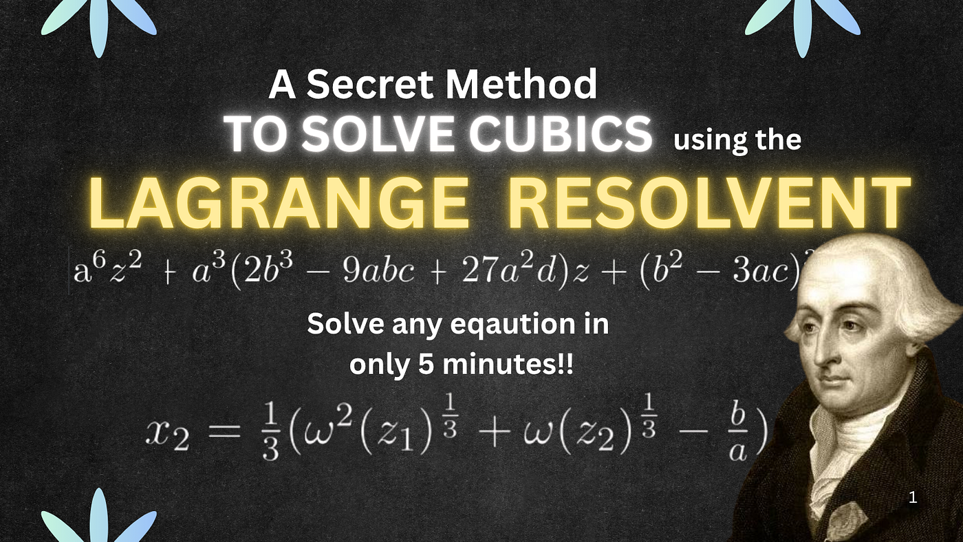
How would Lagrange solve the general cubic?

Note: Please switch to dark mode for a more immersive experience.

1.1 Introduction

We have come across many methods to solve cubics by now. The factoring method, the numerical methods, or even folding some paper.

But I feel that something was missing there. None of those methods give you the feel of taking any random cubic equation and finding the exact form solution using just your pen and paper.

The same feeling you get when using the quadratic formula, you know?

So today, I will be discussing a very interesting, almost unheard-of method of solving general cubic equations using a method developed by the Italian-French mathematician and physicist Joseph-Louis Lagrange.

Using the Lagrange Resolvent method, you will solve these equations in a fashion you’ve never seen before;

By simply finding the roots of a quadratic equation and abusing hidden symmetries in the cubic!

Want to see how?

1.2 Algorithm

I feel like beginning today with a nice little demonstration will help it sink in better.

Then, afterwards we will deeply discuss the way it ticks in the background.

So, the cubic we will be using today is:

And these are its three roots, which we will try to match with our method:

Next, we will move on to the ‘resolvent’ part of our method.

For any cubic equation of the general form, ax³ + bx² + cx + d = 0, its resolvent quadratic is given by the following formula in terms of the coefficients:

I get it's a bit big — but the work it will put in for us is wondrous!

This is a quadratic equation in a variable z ( just to keep it distinct from x) and will yield two roots for us, say z_1 and z_2.

These roots become the key to finding the roots of the cubic later on.

So for the cubic in our case, let's go ahead and plug our numbers in and find this resolvent equation:

Which, after a small simplification, turns into the following:

The formula is just scary because there's a bunch of crazy powers of a, b, and c; however, once you realize they are just constants at the end of the day, it becomes pretty simple.

Then, we can use our trusted quadratic formula to find the roots z_1 and z_2 of this resolvent as:

Make sense until now? Next, we will write down the exact roots of the cubic. We have formulas that look like this:

Here, the letter ω (omega) represents the complex cube root of unity, such that:

Doesn’t that just work like magic??

If you have any questions about why what is what, hold on, because we will be deriving all three of these later. The real fun is in that background work indeed!

Well, let's plug in our roots z_1 and z_2 into these to obtain the final answers to our cubic as:

In one swoop, we have all three exact-form answers.

To confirm we do have the correct roots, let’s plug these values into Wolfram Alpha and get the decimal forms as:

Make sure you use the cbrt() function when plugging in the roots or else it will give other answers.

It works!!

So we have now shown that this algorithm, wherever it comes from, definitely finds and gives us the exact answer to the cubics — in minimal steps!

I'm sure you want to see how it actually works, right?

1.3 Exploiting the beautiful symmetry

The magic of this method actually lies deeply in the properties of the complex cube roots of 1 ( ω and ω²).

So, let’s go ahead and talk about some properties that we will later use in this derivation.

First, we start with the equation:

We put them equal to zero one by one. The first factor gives us the real answer as x = 1.

But our interest is in the remaining quadratic, whose roots are ω and ω².

This is not a notation thing; This value is the square of the ω value in the first picture. You can verify it using the product of roots as well

So, if we talk about the properties, the most obvious one is that ω³ = 1, because it's a cube root of unity.

Moreoever, since it is also the root of x² + x + 1 = 0, it must satisfy the equation as:

This one is going to help us a lot as well when we try to derive the resolvent quadratic later on.

Alright, let's switch gears and focus on the thing that Lagrange first noticed when making this method.

And it involves a very beautiful use of symmetry with the roots.

Say you have a cubic equation of the general form ax³ + bx² + cx + d = 0 with the roots as x_1, x_2, and x_3.

I wish to define two quantities on which we will be doing interesting observations, namely:

Here you can notice that M is simply L, but x_3 and x_2 are switched.

Let’s start asking ourselves questions then.

First, what does the order x_1, x_2, x_3 entail? Does it mean x_2 > x_1, or otherwise?

Nothing, right? They are simply placeholder symbols for the actual roots and have zero connection to their actual values.

As such, when you see the expressions from Vieta’s formula like:

These are symmetric expressions. I.e., they are unaffected by naming one root as x_3, x_1, or whatever, so long as their structure is maintained.

If, say, I wanted to name the real root of a cubic as x_3, I could do that; then in the next line I could name it x_1, that won’t change anything.

Another way you can understand this is that each root is treated equally; there are no extra coefficients or powers on any of them — if x_2 is multiplied by the other two roots, so is x_3 in the same manner.

And this symmetry is exactly what allows us to write their values in simple expressions in terms of the polynomial’s coefficients.

Another point to note here is that these values are constant for a given polynomial.

I.e., finding the symmetric sum of the three roots is infinitely easier than actually finding the roots separately.

If you’ve understood that, then the genius behind the earlier values of L and M will soon be apparent to you.

Let’s bring them up again:

M is chosen as the value that is made when x_2 and x_3 are swapped.

At first glance, It's obvious that these expressions in the roots are not at all symmetric. Since we have multiplied ω and ω² by them, they are no longer “equal.”

As such, if I swap the roots, like x_1 for x_2, it will surely change the value expression.

How about we go one step further and see how exactly it will change the value?

Before we do that, though, I wish to define how we are going to be “swapping” or “mixing” the roots, as that is important to our method.

Now, for 3 roots, there are exactly 6 (3!) ways to arrange them.

Now, each of these permutations can be defined by one of the two actions:

1. Ordered Cycling of roots

2. Swapping two roots and leaving the third.

Let’s also see visualizations for each of these:

Here, you can see that cycling basically means to predictably “shift” the roots. 1 goes to 2, 2 goes to 3, and 3 goes back to 1, and so on. This covers 3 of the 6 possible permutations.

Next, we see the other possibility as:

Here, we pick any two roots and leave the third one where it is, which gives us the next three possible permutations.

Note: You can generate all the combinations by applying once (or repeating) one of these on the base order. You will not need to do cycling and then swapping for anyone. Understanding this is part of our argument later.

ABC -> ABC, CAB, BCA, ACB, CBA, BAC

Since everything is nice and defined now, let's actually see what happens when we perform these movements on the value of L.

So, L is here:

Now, I am going to first apply a cyclic change to the roots, and let's call the new version of L as L ’.

Then:

We have to closely look at L’. Consider the fact that ω³ = 1

After a bit of thinking, maybe you would’ve reached this:

Even without writing the steps down, this is very obvious even visually, right?

I we shift the roots one more time, say that new expression is L’’ and that can trivially be reduced to:

This should have made sense? Now, here is the big master step we need to make.

What happens if we cube these expressions?

Well, the results are pretty clean:

Because ω³ = ω⁶ = 1, the omega factor vanishes upon cubing, telling us that the cubes of all three arrangements of the roots are the exact same!

In a very similar fashion, we can also consider the effects when roots are permutated the other way.

I.e., if in L, we swapped x_1 and x_2 and called the new value M’, what do we get?

If we sit and think about this another similar way (compare it to the value of M all the way up there), we should get the following expression:

And similarly, when we do one more permutation and cube all the expressions together, we get another similar expression as:

This time, because ω⁶ = ω¹² = 1, the omega factor vanishes upon cubing, so again, the cubes of all these three arrangements of roots are also the same!

Are you following along until here? It’s a very interesting concept and really brings forward why it is so interesting and genius!

You might've noticed: alright, so for the cyclic changes L³ remains constant, and for the other type of changes, M³ remains constant.

Cool, but how do M and L change together? What I meant to say is that in isolation they work fine, but what happens to M if I cyclically change the roots? Or vice versa?

Well lets see what actually happens with a simple example:

Consider your roots are in the order ABC, then your L and M look like:

Say I cyclically changed the order of the roots to CAB, then we get:

Here L’ = ωL and M’ = ω²M, right? So by our argument earlier, (L’)³ = L³ and (M’)³ = M³, the values remain perfectly identical

Whenever you make a cyclic transformation, one of L or M will get multiplied by ω and one of them by ω², hence when we cube it, that flies away!

In the same flow, I also want to discuss what happens when we do a non-cyclic transformation to the original roots, i.e., consider the order as ACB.

This gives us the following values:

Another interesting thing has happened here! L’ and M’ are simply the swapped values of L and M!

Thus, now here, (L’)³ = M³ and (M’)³ = L³ !!

And that is how we bring together all the logic.

1. We saw that when we made cyclic changes to L and cubed the resultants, the values all came to be L³
2. We saw that when we made non-cyclic changes to L, all the values came out to be M³
3. We then saw that when we consider both L and M in action and perform the changes, two things can happen:

• For a cyclic change, both L³ and M³ remain exactly their respective values. The cyclic shift simply multiplies one of them by ω and the other by ω², so cubing them vanishes that.
• For a non-cyclic change, it is simpler, as L and M simply swap places.

This all logic culminates in one fact:

For a cubic equation, L³ and M³ are constant values; max to max, they will swap their places if you consider the roots in a certain different order.

The next small logic we will apply is that to overcome that one case where L³ and M³ may change values (by swapping), we may simply use symmetric operations like addition and multiplication.

*Thus, we can say that L³ + M³ and L³ M³ are constant values for any cubic equations, no matter what order the roots are considered in.**

I hope you understand why we had to prove so many results here just to start the derivation.

Let's get back to the start of this argument and bring it full circle.

I said that when you have symmetric expressions, they can be easily written in terms of the coefficients of the polynomials(as constants), like in Vieta’s formulas, but since they treat every root as the same, we cannot isolate any one value.

However, that could be possible if the expression was not symmetric.

Now, we have found L and M that are not symmetric at all to the roots.

And then *L³ + M³ and L³ M ³ **exist, which are symmetric as they don’t care in which order the roots are taken.

Francois Vieta’s work tells us that any symmetric expression in terms of the polynomial’s roots can be written as an expression involving only its coefficients.

Starting to see why this is a very interesting and smart way to abuse this math concept?

This dichotomy will become the reason we can create the resolvent quadratic and even find the roots later!

1.4 Putting it all together.

Until now you’ve seen those two formulas, right? Let’s try to derive them one by one at a time.

The first one we shall do is the resolvent quadratic itself, because that's the real hefty one.

First of all, what is it and where does it come from?

The resolvent quadratic is made from the idea that L³ + M³ and L³ * M³ are constant for a given cubic.

Now, if you know the sum of two numbers and their product, you can construct a quadratic equation to find their values, can't you??

That is exactly what it is:

Keep asking yourself questions! Why can I say this is the resolvent for the cubic itself and not when the roots are taken in a specific order?

Because they are perfectly symmetric expressions! Yes, you got it!

The next step is to represent this in terms of the coefficients, right? The values of L³ and M³ won't come to you in a dream!

The way we will do that is to first consider the values of L + M and LM, then work our way up to L³ + M³ and L³M³ using algebraic identities and cubing.

I recommend you take a piece of paper and try to do this by yourself and soon realise a certain fact — it's pretty tough.

While not impossible, when you consider the whole cubic equation and try to use Vieta’s formulas to find an expression in terms of the coefficients, it gets very difficult.

The way I am going to show here is going to involve ‘depressing’ the cubic, which means making the x² term disappear, and that will make it way easier.

I won’t go into it very deeply, but we depress a cubic of the form ax³ + bx² + cx + d = 0 by using the following substitution:

i is just for representing the difreent roots; you can just put x and y

So, when we apply this to the general cubic we have been considering this whole time (did you remember?), we end up with this:

Just expand and group terms

I also decided to divide the coefficient for some cleanliness.

Here, y_1, y_2, y_3 are the roots of the cubic, and they are just shifted versions of x_1, x_2, and x_3.

Another thing is: how can we use this equation to find the values of L and M when its roots are not the same? (They are shifted)

I recommend you go ahead and place the expression y_i - b/3a where you see x_i in the L and M formula.

You will not take long to realise that the value will not change at all.

Note: Try using the identity ω² + ω + 1 = 0

So, we will find the values using this smaller equation and then use it to skip the algebra from the larger equation!

One important fact that will help us is that y_1 + y_2 + y_3 = 0.

Let’s begin now!

I’ll call the coefficient of y as P and the constant term as Q for ease of writing.

First, we look at the value of L + M, which comes out to be:

Using the identity that ω + ω² + 1 = 0, we have that ω + ω² = -1

Using that in the expression:

We used that y_1 + y_2 + y_3 = 0 to make that substitution in step 3.

Don’t be scared by seeing just one root in the value for L + M, which we obviously cannot describe in terms of a b c d.

That will sort itself out later; let's focus on LM.

When we similarly expand the value LM, we end up with something like this:

Simply realise that the expression is the sum taken two at a time of the cubic and the value is hence simply P ( for y³ + Py + Q = 0, which we are considering right now) and also that ω + ω² = -1.

Using these facts, we end up with:

And this is the second expression we needed, expressed perfectly in terms of the coefficients.

Now, we need to make their bigger siblings, namely L³ + M³ and L³ * M³!

For the latter it's pretty simple; we just cube this last equation to get the following:

Next, to find L³ + M³, we use the following algebraic identity:

We simply plug the values we found into this to get:

Here, we cleverly were able to write y_1³ + Py_1 = -Q because it was the root of the cubic y³ + Py + Q = 0.

Thus, we finally get the values of the magic, symmetric terms as:

Ahh, that took long but could've been 10x longer if not for our trick of depressing the equation.

Anyhow, let's put this back into our formula for the resolvent quadratic to get the expression in terms of a b c d.

So we end up getting:

And then if we put the value of P and Q from earlier:

Now, we are a simple LCM taking away from getting the equation I showed at the start of the discussion, which was:

Also flipped the 3ac-b² term for the plus sign.

And there you have it! A complete derivation of the resolvent quadratic!

By definition, the roots of this quadratic equation are L³ and M³, right?

And this quadratic has nice constant coefficients, so we can definitely find those roots.

Hence, the next thing to do is to connect the roots of the quadratic to the ones of the cubic eqaution!

That is a very trivial thing done using a very simple high school-level concept.

We will consider the following three equations we know in terms of the original roots x_1, x_2, and x_3, which are:

Now, see what happens when you add all three equations:

The RHS becomes:

And the RHS gives you the following:

Because 1 + ω + ω² = 0

Thus, we can isolate x_1 as:

Beautiful, isn't it?

The concept there is that the one without ω in all three equations is the one that survives! So, we isolate x_2 and x_3; we just multiply the L and M with ω until they become free.

And this way, we have also reached the formula we had looked at so puzzlingly at the start today.

1.5 Conclusion

And there you have it! What seemed like totally overpowered black magic at the start is actually just a beautiful dance of symmetry.

By abusing the properties of ω, Lagrange figured out how to bundle those messy roots into a simple quadratic and perfectly unpack the exact answers. The crazy part? This exact idea of playing with root symmetries actually laid the groundwork for Galois theory and changed math forever.

Pretty overpowered for just pen and paper, right?

See y’all next week!