Pandas in Python — Part 1 🐼

Photo by Sid Balachandran on Unsplash

Pandas is one of the most powerful and widely used Python libraries for data manipulation, analysis, and visualization. It provides flexible and efficient data structures, mainly Series and DataFrame, which make working with structured data simple and intuitive.

⚡Pandas is a powerful and flexible open-source data analysis and manipulation library for Python. It is built on top of the NumPy library and provides data structures like Series and DataFrame, which are designed to work efficiently with structured data.

⚡It has functions for analyzing, cleaning, exploring, and manipulating data.

⚡The name “Pandas” is a reference to both “Panel Data” and “Python Data Analysis” and was created by Wes McKinney in 2008.

🔥 Introduction to Pandas

Pandas is built on top of NumPy, meaning it works efficiently with numerical data and integrates well with scientific computing in Python. It provides easy handling of tabular data, similar to Excel or SQL tables.

🛠 Installation

If you haven’t installed Pandas yet, you can install it using pip:

pip install pandas

Once installed, import it:

import pandas as pd

1. Pandas Data Structures

Pandas provides two primary data structures for managing data: Series and DataFrame. Both are built on top of NumPy arrays but provide more powerful features, particularly for data analysis tasks.

✅ 1.1 Pandas Series (1D Data)

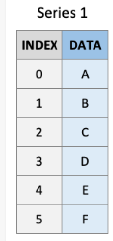
A Series is a one-dimensional array-like object that holds a sequence of values along with an associated index.

⚡A Series is a one-dimensional labeled array capable of holding any data type (integers, strings, floats, Python objects, etc.). It is similar to a column in a spreadsheet or a single column in a DataFrame.

Key Characteristics:

⚡Indexing: Each element in a Series has an associated label, known as its index.

⚡Homogeneous Data: A Series is homogeneous, meaning it can hold data of only one type.

📌 Creating a Pandas Series

import pandas as pd

# Creating a Series from a list
data = [10, 20, 30, 40, 50]
s = pd.Series(data)

print(s)

⏳Output:

0    10
1    20
2    30
3    40
4    50
dtype: int64

Each value has an index assigned automatically (starting from 0). You can also set custom indexes.

s = pd.Series(data, index=['a', 'b', 'c', 'd', 'e'])
print(s)

📌 Accessing Series Elements

print(s['b'])  # Output: 20
print(s[1])    # Output: 20

If you have custom string-based indexes (['a', 'b', 'c', 'd', 'e'] in your case),

• s[1] currently retrieves the value by position (zero-based index).
• In future versions, s[1] will be treated as accessing an index label (which may not exist).
• Instead of s[1]Use s.iloc[1]

print(s.iloc[1])  # ✅ Always retrieves by position (2nd element)

✅ 1.2 Pandas DataFrame (2D Data)

A DataFrame is a two-dimensional table with labeled rows and columns.

⚡A DataFrame is a two-dimensional, size-mutable, and potentially heterogeneous tabular data structure with labeled axes (rows and columns). It is similar to a spreadsheet or SQL table, or a dictionary of Series objects.

Key Characteristics:

⚡Indexing: Both rows and columns are indexed, allowing for easy access and manipulation.

⚡Heterogeneous Data: Each column in a DataFrame can contain different data types (e.g., integers, floats, strings).

⚡Size-Mutable: The size of the DataFrame can be changed (adding/removing rows or columns).

📌 Creating a DataFrame

# Creating DataFrame from a dictionary
data = {
    'Name': ['Alice', 'Bob', 'Charlie'],
    'Age': [25, 30, 35],
    'Salary': [50000, 60000, 70000]
}

df = pd.DataFrame(data)

print(df)

# Creating a DataFrame from a list of lists
df = pd.DataFrame([[1, 2], [3, 4]], columns=['A', 'B'])

⏳Output:

#DataFrame from a dictionary
     Name  Age  Salary
0   Alice   25  50000
1     Bob   30  60000
2  Charlie   35  70000

#DataFrame from a list of lists
   A  B
0  1  2
1  3  4

📌 Accessing Data

print(df['Name'])      # Accessing a column
print(df.loc[1])       # Accessing a row by label
print(df.iloc[1])      # Accessing a row by position

⏳Output:

0      Alice
1        Bob
2    Charlie
Name: Name, dtype: object

Name        Bob
Age          30
Salary    60000
Name: 1, dtype: object

Name        Bob
Age          30
Salary    60000
Name: 1, dtype: object

📌 Difference Between loc[] and iloc[] in Pandas

Both **loc[] and iloc[] are used to access rows in a Pandas DataFrame**, but they differ in how they reference rows.

📌 Adding a New Column

df['Experience'] = [2, 5, 8]
print(df)

#Output:
   Name  Age  Salary  Experience
0    Alice   25   50000           2
1      Bob   30   60000           5
2  Charlie   35   70000           8

📌 Deleting a Column

df.drop('Salary', axis=1, inplace=True)
print(df)

This line removes the column named "Salary" from the DataFrame df.

‘Salary’ → The name of the column to be dropped.

axis=1 → Specifies column removal (use axis=0 for row removal).

inplace=True → Modifies df directly instead of returning a new DataFrame.

⏳Output:

      Name  Age  Experience
0    Alice   25           2
1      Bob   30           5
2  Charlie   35           8

🚨 Important Notes

**inplace=True modifies the DataFrame directly.**

If inplace=False (default), it returns a new DataFrame instead of modifying df.

For multiple column deletion, pass a list:

df.drop(['Salary', 'Age'], axis=1, inplace=True)

To drop rows instead of columns, use axis=0:

df.drop(1, axis=0, inplace=True)  # Removes row with index 1 (Bob)

📌 Filtering Data

print(df[df['Age'] > 25])

#Output:
    Name  Age  Experience
2  Charlie   35           8

📌Viewing the Index

print(df.index)

The command **print(df.index)** prints the index of a Pandas DataFrame.

⏳Output:

RangeIndex(start=0, stop=3, step=1)

This means the DataFrame has a default integer index starting from 0 to 2.

🔹 If you have a custom index:

df.index = ['A', 'B', 'C']
print(df.index)

⏳Output:

Index(['A', 'B', 'C'], dtype='object')

This shows that the index now consists of custom labels.

📌Accessing columns of a DataFrame

print(df.columns)

It returns an Index object listing all column names in your DataFrame.

⏳Output:

Index(['Name', 'Age', 'Salary'], dtype='object')

🔹If You Want Column Names as a List:

column_list = df.columns.tolist()
print(column_list)  # Output: ['Name', 'Age']

✅Basic Operations on DataFrames in Pandas

1️⃣Viewing Data

Pandas provides methods to preview data quickly.

Create a dataframe

import pandas as pd

# Creating a dictionary with data
data = {'Name': ['Alice', 'Bob', 'Charlie'],
        'Age': [25, 30, 35],
        'City': ['New York', 'London', 'Paris']}

# Creating a DataFrame from the dictionary
df = pd.DataFrame(data)

print(df)

🔹 Example: Displaying the first few rows

print(df.head(2))  # Show the first 2 rows

⏳Output:

     Name  Age      City
0   Alice   25  New York
1     Bob   30    London

.head(n) displays the first n rows of the DataFrame.

If n is not specified, it defaults to 5.

🔹Viewing the Last Few Rows

The .tail(n) method is used to display the last n rows of a DataFrame. If n is not provided, it defaults to 5.

# Display the last 2 rows
print(df.tail(2))

⏳Output:

      Name  Age    City
1      Bob   30  London
2  Charlie   35   Paris

.tail(n) shows the last n rows of the DataFrame.

If n is not specified, it will return the last 5 rows by default.

2️⃣ Selecting Data

Selecting data from a Pandas DataFrame is a fundamental operation that allows you to filter, slice, and manipulate your data based on specific criteria. Pandas provides various ways to select data from a DataFrame, including by column, row, index, and using conditions.

🔹 Example: Selecting a single column

print(df['Name'])

⏳Output: Returns a Series (one-dimensional array) containing all values from the Name column.

0     Alice
1       Bob
2  Charlie
Name: Name, dtype: object

🔹 Example: Selecting multiple columns

print(df[['Name', 'City']])

⏳Output: Pass a list of column names to select multiple columns.

     Name      City
0   Alice  New York
1     Bob    London
2  Charlie     Paris

🔹Example: Selecting a row by index

print(df.loc[1])  # Select row with index 1

⏳Output: .loc[] selects a row by label-based indexing.

Name      Bob
Age        30
City    London
Name: 1, dtype: object

🔹 Example: Selecting a row by position

print(df.iloc[1])  # Select row at position 1

⏳Output: .iloc[] selects a row by integer position.

Name      Bob
Age        30
City    London
Name: 1, dtype: object

3️⃣Filtering Data

Filtering data in Pandas involves selecting subsets of data that meet specific conditions. This is a powerful way to focus on the most relevant data for analysis based on criteria like column values, data types, or custom logic.

You can filter rows based on conditions.

🔹 Example: Filtering rows where Age > 28

print(df[df['Age'] > 28])

⏳Output:

     Name  Age   City
1     Bob   30  London
2  Charlie   35   Paris

The condition df['Age'] > 28 creates a Boolean mask (True or False).

Only rows where the condition is True are displayed.

🔹Example: Applying multiple conditions

Use logical operators like & (AND), | (OR), and ~ (NOT) to combine multiple conditions. Enclose each condition in parentheses.

df[(df['Age'] > 25) & (df['City'] == 'London')] # Both conditions must be True

⏳Output:

Name Age City
1 Bob 30 London

& is used for AND conditions.

| can be used for OR conditions

🔹More Examples :

df[(df['Age'] < 35) | (df['Name'] == 'Alice')]  # Either condition can be True

⏳Output:

 Name Age City
0 Alice 25 New York
1 Bob 30 London

🔹More Examples :

# Selects all rows where 'Name' is not 'Bob'
df[~(df['Name'] == 'Bob')] 

⏳Output:

 Name Age City
0 Alice 25 New York
1 Bob 30 London

📌Filtering Data in Pandas Using isin()

The isin() function in Pandas is used to filter rows based on whether a column's values match a list or set of values. It is useful when you want to select specific categories, labels, or numerical values from a DataFrame.

🔹Syntax of isin()

df[df['column_name'].isin([value1, value2, value3])]

✔️Keeps rows where column_name matches one of the given values. ✔️ Returns a new filtered DataFrame.

🔹Example 1: Filtering Rows Based on Multiple Values

import pandas as pd

# Sample DataFrame
data = {
    'Name': ['Alice', 'Bob', 'Charlie', 'David', 'Eve'],
    'Age': [25, 30, 35, 40, 28],
    'City': ['New York', 'Paris', 'London', 'New York', 'Berlin']
}
df = pd.DataFrame(data)
print("Original DataFrame:\n", df)

# Filtering: Select people who are from 'New York' or 'London'

filtered_df = df[df['City'].isin(['New York', 'London'])]
print("\nFiltered DataFrame:\n", filtered_df)

⏳Output:

Original DataFrame:
      Name  Age      City
0  Alice   25  New York
1    Bob   30     Paris
2 Charlie   35   London
3  David   40  New York
4    Eve   28   Berlin

Filtered DataFrame:
      Name  Age      City
0  Alice   25  New York
2 Charlie   35   London
3  David   40  New York

Only rows where City is 'New York' or 'London' are kept.

🔹Example 2: Filtering Rows Using a List of Values

# Filtering people with Age 25 or 40
filtered_df = df[df['Age'].isin([25, 40])]
print(filtered_df)

⏳Output:

    Name  Age    City
1    Bob   30   Paris
4    Eve   28  Berlin

Keeps only rows where Age is either 25 or 40.

🔹Example 3: Filtering Rows That Do Not Match Values (~isin())

# Exclude rows where City is 'New York' or 'London'
filtered_df = df[~df['City'].isin(['New York', 'London'])]
print(filtered_df)

⏳Output:

    Name  Age    City
1    Bob   30   Paris
4    Eve   28  Berlin

Using ~ (NOT operator), we remove 'New York' and 'London'.

🔹Example 4: Using isin() with Multiple Columns

# Filtering rows where either Name is 'Alice' or Age is 40
filtered_df = df[df['Name'].isin(['Alice']) | df['Age'].isin([40])]
print(filtered_df)

⏳Output:

    Name  Age      City
0  Alice   25  New York
3  David   40  New York

Keeps rows where either Name is 'Alice' OR Age is 40.

📌 Filtering Data Using between() in Pandas

The between() function in Pandas filters values within a specified range (inclusive of both ends). It is mainly used for filtering numeric values and dates.

🔹 Syntax of between()

df[df['column_name'].between(lower_value, upper_value)]

✔️Keeps rows where column_name is between lower_value and upper_value (inclusive). ✔️Works for numerical and datetime values.

🔹Example 1: Filtering Numbers Using between()

import pandas as pd

# Sample DataFrame
data = {
    'Name': ['Alice', 'Bob', 'Charlie', 'David', 'Eve'],
    'Age': [25, 30, 35, 40, 28],
    'Salary': [50000, 60000, 70000, 80000, 90000]
}
df = pd.DataFrame(data)

# Filtering rows where Age is between 28 and 35
filtered_df = df[df['Age'].between(28, 35)]
print(filtered_df)

⏳Output:

    Name  Age  Salary
1    Bob   30  60000
2 Charlie   35  70000
4    Eve   28  90000

Only rows where Age is between 28 and 35 (inclusive) are kept.

🔹Example 2: Filtering Dates Using between()

# Creating a DataFrame with dates
df['Join_Date'] = pd.to_datetime(['2022-01-10', '2023-03-15', '2023-06-25', '2024-02-20', '2024-04-05'])

# Filtering employees who joined between '2023-01-01' and '2023-12-31'
filtered_df = df[df['Join_Date'].between('2023-01-01', '2023-12-31')]
print(filtered_df)

⏳Output:

    Name  Age  Salary  Join_Date
1    Bob   30  60000 2023-03-15
2 Charlie   35  70000 2023-06-25

Filters only employees who joined in 2023.

🔹Example 3: Using between() with inclusive Parameter

By default, between() includes both ends of the range (inclusive='both'). You can change it to exclude the boundaries:

# Exclude 28 and 35 from the filter
filtered_df = df[df['Age'].between(28, 35, inclusive='neither')]
print(filtered_df)

⏳Output:

    Name  Age  Salary
1    Bob   30  60000

Now, 28 and 35 are excluded.

🔹Example 4: Using ~between() to Exclude a Range

# Exclude employees with Salary between 60000 and 80000
filtered_df = df[~df['Salary'].between(60000, 80000)]
print(filtered_df)

⏳Output:

    Name  Age  Salary
0  Alice   25  50000
4    Eve   28  90000

Keeps only salaries outside the range 60,000–80,000.

📌Filtering Rows in Pandas Based on String Matching

Filtering string-based columns in Pandas is useful when working with names, categories, or text fields. We can do this using:

✅ String Matching (str.contains(), str.startswith(), str.endswith())

🔹Example: Using str.contains() for Partial Matches

str.contains() is useful for finding substrings within a column.

import pandas as pd

# Sample DataFrame
data = {
    'Name': ['Alice', 'Bob', 'Charlie', 'David', 'Eve'],
    'City': ['New York', 'Los Angeles', 'London', 'Berlin', 'New Delhi'],
    'Age': [25, 30, 35, 40, 28]
}
df = pd.DataFrame(data)

# Filter rows where 'City' contains 'New'
filtered_df = df[df['City'].str.contains('New', case=False)]  # case=False makes it case-insensitive
print(filtered_df)

⏳Output:

    Name  City        Age
0  Alice  New York    25
4    Eve  New Delhi   28

Keeps only rows where "City" contains "New".

🔹Example: Using str.startswith()

# Rows where 'City' starts with 'New'
df[df['City'].str.startswith('New')]

⏳Output:

    Name  City        Age
0  Alice  New York    25
4    Eve  New Delhi   28

🔹Example: Using str.endswith()

# Rows where 'City' ends with 'n'
df[df['City'].str.endswith('n')]

⏳Output:

    Name  City   Age
3  David  Berlin  40

Useful for filtering names, locations, or categories that start or end with a specific string.

🔹Example: Using Regex in str.contains()

# Find cities that start with 'New' or 'Los'
df[df['City'].str.contains(r'^(New|Los)', regex=True)]

⏳Output:

    Name  City          Age
0  Alice  New York      25
1    Bob  Los Angeles   30
4    Eve  New Delhi     28

Regex allows more advanced pattern matching.

📌Filtering Rows in Pandas Based on query()

The **query() function provides a SQL-like syntax** for filtering.

🔹Example: Filtering Using query()

df_filtered = df.query("Age > 30")
print(df_filtered)

⏳Output: Filters rows where Age is greater than 30.

    Name  City    Age
2  Charlie  London  35
3  David    Berlin  40

🔹Example: Using query() with Multiple Conditions

df_filtered = df.query("Age > 25 & City == 'London'")
print(df_filtered)

⏳Output: Filters rows where Age is greater than 25 AND City is 'London'.

    Name   City    Age
2  Charlie  London  35

4️⃣Adding & Modifying Columns

We can add new columns or modify existing ones.

🔹 Example: Adding a new column

df['Salary'] = [50000, 60000, 70000 , 40000, 50000]
print(df)

⏳Output:

     Name  Age      City  Salary
0   Alice   25  New York  50000
1     Bob   30    London  60000
2  Charlie   35     Paris  70000

A new column Salary is added with respective values.

🔹Example: Modifying an existing column

df['Age'] = df['Age'] + 1
print(df)

⏳Output:

     Name  Age      City  Salary
0   Alice   26  New York  50000
1     Bob   31    London  60000
2  Charlie   36     Paris  70000

Every age value is increased by 1

5️⃣Deleting Columns & Rows

🔹 Example: Removing a column

df.drop(columns=['Salary'], inplace=True)
print(df)

⏳Output:

     Name  Age      City
0   Alice   26  New York
1     Bob   31    London
2  Charlie   36     Paris

inplace=True modifies the DataFrame directly.

🔹 Example: Removing a row

df.drop(index=1, inplace=True)
print(df)

⏳Output:

     Name  Age      City
0   Alice   26  New York
2  Charlie   36     Paris

The row with index 1 is removed.

6️⃣ Sorting Data

We can sort the DataFrame based on column values.

🔹 Example: Sorting by Age

print(df.sort_values(by='Age', ascending=False))

⏳Output:

     Name  Age      City
2  Charlie   36     Paris
0   Alice   26  New York

Sorts the DataFrame by Age in descending order

7️⃣Grouping & Aggregations

🔹Example: Average age per city

print(df.groupby('City')['Age'].mean())

⏳Output:

City
New York    26.0
Paris       36.0
Name: Age, dtype: float64

Groups data by City and calculates the average Age.

8️⃣Handling Missing Data

🔹 Example: Checking for missing values

import pandas as pd

# Sample DataFrame
data = {
    'Name': ['Alice', 'Bob', 'Charlie', 'David', None],
    'City': ['New York', 'Los Angeles', None, 'Berlin', 'New Delhi'],
    'Age': [25, 30, 35, None, None]
}
df = pd.DataFrame(data)

print(df.isnull().sum())  # check for null values

⏳Output:

Name    1
Age     1
City    2  
dtype: int64

🔹Example: Filling missing values

df.fillna(value={'Age': 99}, inplace=True)
print(df)

⏳Output: Replaces NaN values in Age with 99.

 Name City Age
0 Alice New York 25.0
1 Bob Los Angeles 30.0
2 Charlie None 35.0
3 David Berlin 99.0
4 None New Delhi 99.0

🔹Example: Dropping Missing Values: dropna()🗑️

The .dropna() method is used to remove rows or columns that contain missing (NaN) values in a DataFrame.

🔹Example 1: Dropping Rows with Missing Values

import pandas as pd
import numpy as np

# Creating a DataFrame with missing values (NaN)
data = {'Name': ['Alice', 'Bob', 'Charlie', 'David'],
        'Age': [25, np.nan, 35, 40],
        'City': ['New York', 'London', np.nan, 'Berlin']}

df = pd.DataFrame(data)

# Dropping rows with any NaN values
df_cleaned = df.dropna()

print(df_cleaned)

⏳Output:

    Name   Age     City
0  Alice  25.0  New York
3  David  40.0   Berlin

The .dropna() method removes rows where any column contains a NaN (missing value).

In this case:

Row 1 (Bob) is dropped because Age is NaN.

Row 2 (Charlie) is dropped because City is NaN.

🔹 Example 2: Dropping Columns with Missing Values

# Dropping columns with any NaN values
df_cleaned_cols = df.dropna(axis=1)

print(df_cleaned_cols)

⏳Output:

    Name
0  Alice
1    Bob
2 Charlie
3  David

axis=1 means columns will be dropped if they contain NaN values.

Both Age and City columns contained missing values, so they were removed from the DataFrame.

🔹 Example 3: Dropping Rows Only If All Values Are Missing

# Creating a DataFrame with a completely empty row
data = {'Name': ['Alice', 'Bob', None, 'David'],
        'Age': [25, np.nan, np.nan, 40],
        'City': ['New York', 'London', np.nan, 'Berlin']}

df = pd.DataFrame(data)

# Dropping rows only if all values are NaN
df_cleaned = df.dropna(how='all')

print(df_cleaned)

⏳Output:

    Name   Age     City
0  Alice  25.0  New York
1    Bob   NaN   London
3  David  40.0   Berlin

The how=’all’ argument ensures that only rows where all values are NaN are removed. In this case: Row 2 is completely empty (None, NaN, NaN) and gets removed. Row 1 has at least one non-null value (London), so it remains.

9️⃣Renaming Columns and Index in Pandas

The .rename() method in Pandas allows you to rename column names and index labels in a DataFrame.

🔹 Example 1: Renaming Column Names

import pandas as pd

# Creating a DataFrame
data = {'Name': ['Alice', 'Bob', 'Charlie'],
        'Age': [25, 30, 35],
        'City': ['New York', 'London', 'Berlin']}

df = pd.DataFrame(data)

# Renaming columns
df_renamed = df.rename(columns={'Name': 'Full Name', 'Age': 'Years'})

print(df_renamed)

⏳Output:

  Full Name  Years     City
0    Alice     25  New York
1      Bob     30   London
2  Charlie     35   Berlin

columns={'Name': 'Full Name', 'Age': 'Years'} → Renames:

"Name" → "Full Name"

"Age" → "Years"

The "City" column remains unchanged

🔹Example 2: Renaming Index Labels

# Renaming index labels
df_index_renamed = df.rename(index={0: 'A', 1: 'B', 2: 'C'})

print(df_index_renamed)

⏳Output:

   Name  Age     City
A  Alice   25  New York
B    Bob   30   London
C  Charlie  35   Berlin

🔹 Example 3: Renaming Columns Using a Function

# Renaming all columns to uppercase
df_uppercase = df.rename(columns=str.upper)

print(df_uppercase)

⏳Output:

     NAME  AGE     CITY
0  Alice   25  New York
1    Bob   30   London
2  Charlie  35   Berlin

🔹Example 4: Renaming Index Using a Function

# Renaming index labels to start from 100
df_index_shifted = df.rename(index=lambda x: x + 100)

print(df_index_shifted)

⏳Output:

   Name  Age     City
100  Alice   25  New York
101    Bob   30   London
102  Charlie  35   Berlin

Thank you so much for reading. Follow me for more content like this.

Happy learning 😊