Single Layer Perceptron (SLP): The Foundation of Neural Networks

Introduction

Artificial Intelligence and Machine Learning have transformed the modern world. At the heart of every deep learning model lies a fundamental building block — the Perceptron. The Single Layer Perceptron (SLP) is the simplest form of an artificial neural network and serves as the foundation upon which all complex neural networks are built. In this article, we will explore what SLP is, how it works, its architecture, learning algorithm, advantages, limitations, and Python implementation.

What is a Single Layer Perceptron?

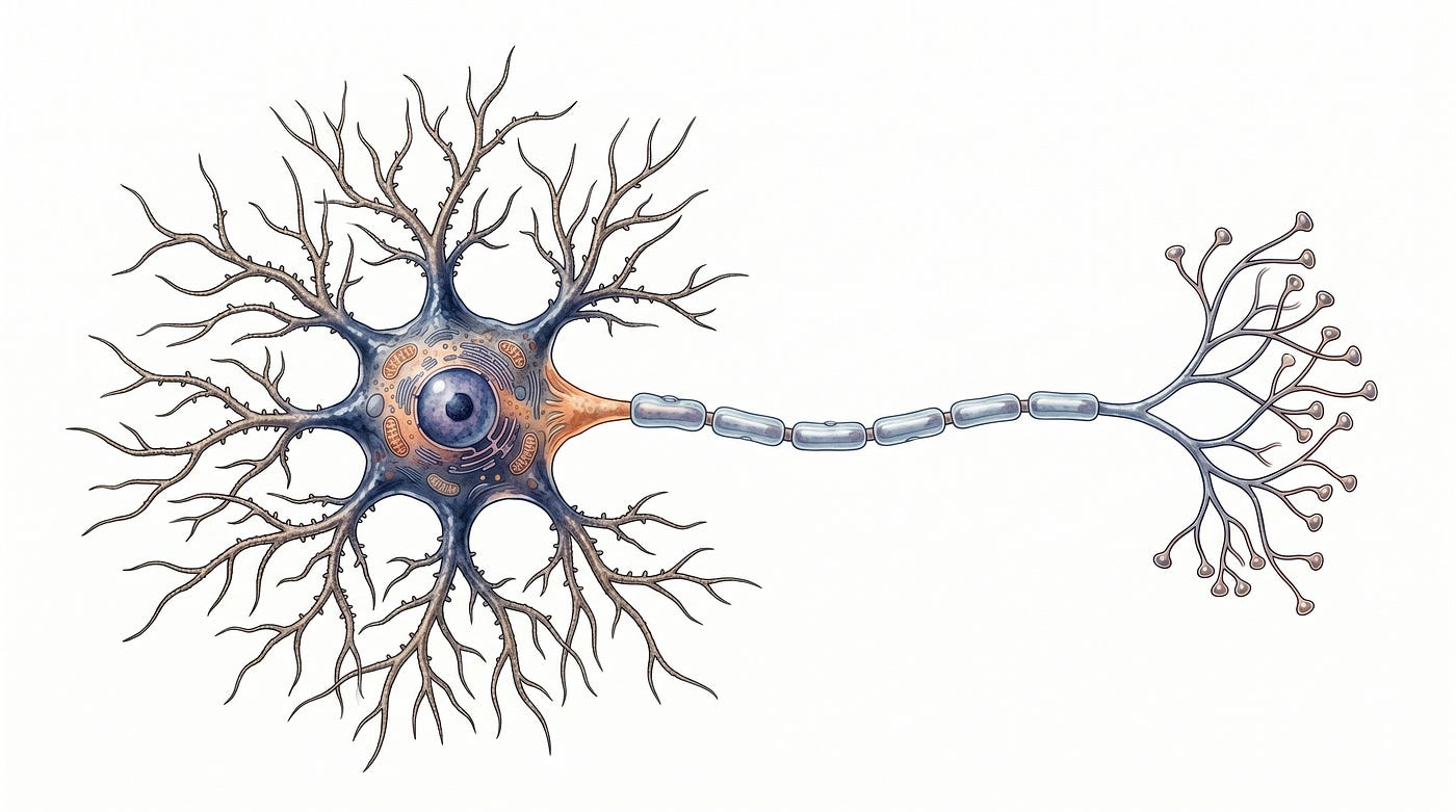
A Single Layer Perceptron (SLP) is the most basic type of artificial neural network. It was introduced by Frank Rosenblatt in 1957 and is inspired by the biological neuron in the human brain. The SLP consists of only one layer of output nodes that are directly connected to the inputs. It is a feed-forward network that processes inputs and produces a binary output based on a threshold activation function.

The SLP can only solve linearly separable problems, meaning it can classify data that can be divided by a straight line (or hyperplane in higher dimensions). Despite this limitation, it laid the groundwork for all modern deep learning architectures.

Architecture of Single Layer Perceptron

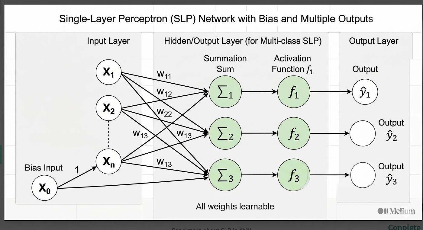
The architecture of a Single Layer Perceptron consists of the following key components:

1. Input Layer: The input layer consists of n input nodes (x1, x2, …, xn). Each input represents a feature of the data. These inputs are fed directly into the neuron.

2. Weights (w1, w2, …, wn): Each input is associated with a weight. Weights determine the importance or contribution of each input to the final output. They are adjusted during the learning process.

3. Bias (b): The bias is an additional input with a fixed value of 1 and its own weight. It helps the model shift the activation function and improves flexibility.

4. Summation Function (Net Input): The net input is computed as the weighted sum of all inputs plus the bias: Net Input = (x1w1 + x2w2 + … + xn*wn) + b

5. Activation Function: The activation function (usually a step function) converts the net input into an output. If net input >= threshold, output = 1; otherwise, output = 0.

6. Output: The final binary output (0 or 1) is produced based on the activation function result.

Photo by notorious v1ruS on Unsplash

How Does a Single Layer Perceptron Learn?

The SLP learns through a process called the Perceptron Learning Algorithm. This is a supervised learning algorithm where the model is trained using labeled data. Here are the steps:

Step 1 — Initialize Weights: Set all weights (w1, w2, …, wn) and the bias (b) to zero or small random values.

Step 2 — Feed Input: For each training sample, feed the input values into the perceptron.

Step 3 — Compute Net Input: Calculate the weighted sum of inputs: Net Input = sum(xi * wi) + b

Step 4 — Apply Activation Function: Apply the step function: If Net Input >= 0, Output (y) = 1 If Net Input < 0, Output (y) = 0

Step 5 — Compute Error: Compare the actual output with the target (desired) output: Error = Target Output — Actual Output

Step 6 — Update Weights: Adjust the weights using the update rule: wi(new) = wi(old) + (learning rate Error xi) b(new) = b(old) + (learning rate * Error)

Step 7 — Repeat: Repeat steps 2–6 for all training samples and multiple epochs until the error is minimized or the model converges.

Python Implementation of Single Layer Perceptron

Here is a simple Python implementation of a Single Layer Perceptron from scratch using NumPy:

import numpy as np

class SingleLayerPerceptron: def init(self, learning_rate=0.1, epochs=100): self.lr = learning_rate self.epochs = epochs self.weights = None self.bias = None

def activation(self, x): return 1 if x >= 0 else 0

def fit(self, X, y): n_samples, n_features = X.shape self.weights = np.zeros(n_features) self.bias = 0

for _ in range(self.epochs): for i in range(n_samples): net_input = np.dot(X[i], self.weights) + self.bias y_pred = self.activation(net_input) error = y[i] — y_pred self.weights += self.lr error X[i] self.bias += self.lr * error

def predict(self, X): return [self.activation(np.dot(x, self.weights) + self.bias) for x in X]

Example: AND Gate

X = np.array([[0,0],[0,1],[1,0],[1,1]]) y = np.array([0, 0, 0, 1]) # AND gate

slp = SingleLayerPerceptron(learning_rate=0.1, epochs=100) slp.fit(X, y) predictions = slp.predict(X) print(‘Predictions:’, predictions)

Advantages of Single Layer Perceptron

1. Simple and Easy to Understand: The SLP is the simplest neural network model. It is easy to implement and understand, making it a great starting point for beginners learning about neural networks and machine learning.

2. Fast Training: Due to its simple architecture and direct computation, the SLP trains very quickly on small datasets.

3. Binary Classification: The SLP is very effective for simple binary classification problems where data is linearly separable.

4. Foundation for Deep Learning: Despite its simplicity, the SLP is the fundamental building block for Multi-Layer Perceptrons (MLP) and all modern deep neural networks.

5. Convergence Guarantee: The Perceptron Convergence Theorem guarantees that if the data is linearly separable, the SLP will converge to a perfect solution in a finite number of iterations.

Limitations of Single Layer Perceptron

1. Cannot Solve Non-Linearly Separable Problems: The biggest limitation of SLP is that it cannot classify data that is not linearly separable. A classic example is the XOR problem, which cannot be solved by a single layer perceptron.

2. Binary Output Only: The SLP produces only binary output (0 or 1), making it unsuitable for multi-class classification problems or regression tasks.

3. No Hidden Layers: The absence of hidden layers means the SLP cannot learn complex features or patterns in the data.

4. Limited Representation Power: Due to its simple architecture, the SLP has very limited representation power and cannot model complex relationships in data.

5. Sensitive to Feature Scaling: The SLP is sensitive to the scale of input features and requires proper feature normalization for effective training.

6. Not Suitable for Complex Real-World Problems: Modern real-world problems such as image recognition, natural language processing, and speech recognition require multi-layer architectures that go far beyond what an SLP can handle.

Conclusion

The Single Layer Perceptron (SLP) is truly the grandfather of modern artificial intelligence and deep learning. Introduced by Frank Rosenblatt in 1957, this simple yet powerful model demonstrated that machines could learn from data and make decisions — a revolutionary concept at the time.

Although the SLP has significant limitations (most notably its inability to handle non-linearly separable problems), it remains an essential concept for anyone studying machine learning and neural networks. Understanding how the SLP works — its architecture, learning algorithm, and weight update mechanism — gives you the foundation you need to understand far more complex models like Multi-Layer Perceptrons (MLP), Convolutional Neural Networks (CNNs), and Recurrent Neural Networks (RNNs).

The journey from a Single Layer Perceptron to modern deep learning models is a testament to how far the field has come. But it all starts here — with one neuron, a few weights, and the desire to learn.

Thank you for reading! If you found this article helpful, feel free to clap, share, and follow for more articles on Machine Learning and Deep Learning.