[Hands-On] Understanding and Implementing Conditional GAN

(You can find the Korean version of the post at this link.)

In the previous post, we delved deeply into the core ideas of GAN (Generative Adversarial Networks). This post is the second in the GAN implementation series, where we will explore the implementation of Conditional GAN (CGAN) in detail and visualize the results. If you feel that your understanding of GANs is not solid, I recommend reading the following two posts before proceeding with this one.

[embed]Understanding GANs Explore the fundamentals, training methods, and applications of Generative Adversarial Networks (GANs) with practical…medium.com

[embed][Hands-On] Understanding and Implementing GANs Learn how to implement and train GANs using PyTorch. Dive into GAN architecture, training methods, and visualize…medium.com

What is CGAN?

A Conditional GAN (CGAN) is a variant of GAN where both the generator and the discriminator receive additional conditional information. This conditional information can be class labels or other forms of data, ensuring that the generated data meets specific conditions.

In simple terms, while the goal of a Basic GAN is to generate any ‘plausible’ image, the goal of a CGAN is to generate a ‘plausible’ image that meets certain conditions.

Think about it; generating something that fits specific conditions is more useful in the real world, right?

Here is a summary of the basic concepts of CGAN:

Key Concepts Summary:

• Conditional Information: Additional information received by both the generator and the discriminator. For example, in the MNIST dataset, the digits from 0 to 9 are used as conditional information.
• Generator: Receives random noise and conditional information as inputs to generate fake data.
• Discriminator: Evaluates both real and fake data along with the conditional information.
• Competitive Learning: The generator and the discriminator learn by competing against each other.

Based on these basic concepts, let’s implement a CGAN.

Preparing the Environment

We will import the libraries necessary for loading data, building the model, training, and evaluation. This step is crucial as it sets up the environment with the tools and libraries needed for specific tasks.

!pip install imageio

import torch
import torch.nn as nn
import torch.optim as optim
from torchvision import datasets, transforms
from torchvision.utils import save_image
import matplotlib.pyplot as plt
import os
import numpy as np

To ensure that our experiments are reproducible, we need to set up a few things.

# Function to set the seed for reproducibility
import random
def set_seed(seed_value=42):
    """Set seed for reproducibility."""
    np.random.seed(seed_value)
    torch.manual_seed(seed_value)
    torch.cuda.manual_seed(seed_value)
    torch.cuda.manual_seed_all(seed_value)  # if you are using multi-GPU.
    random.seed(seed_value)
    os.environ['PYTHONHASHSEED'] = str(seed_value)

    # The below two lines are for deterministic algorithm behavior in CUDA
    torch.backends.cudnn.deterministic = True
    torch.backends.cudnn.benchmark = False

# Set the seed
set_seed()
device = torch.device('cuda' if torch.cuda.is_available() else 'cpu')

Loading the Dataset

In this project, we will use the MNIST dataset, which serves as a “Hello-World” in the realm of machine learning code implementations. The MNIST dataset consists of 70,000 images of handwritten digits (0–9), each with a size of 28x28 pixels.

# DataLoader for MNIST
dataloader = torch.utils.data.DataLoader(
    datasets.MNIST('./data/mnist', train=True, download=True,
                   transform=transforms.Compose([
                       transforms.Resize(28),
                       transforms.ToTensor(),
                       transforms.Normalize([0.5], [0.5])  # Normalize to range [-1, 1]
                   ])),
    batch_size=64, shuffle=True)

transforms. Normalize([0.5], [0.5]) command scales the final output values to be between [-1, 1].

Implementing CGAN Neural Network

A CGAN, like a GAN, consists of a generator and a discriminator. The key difference lies in how conditional information is applied to each neural network.

Generator

class Generator(nn.Module):
    def __init__(self):
        super(Generator, self).__init__()
        self.embedding = nn.Embedding(10, 10)  # Embedding for 10 classes
        self.model = nn.Sequential(
            nn.Linear(100 + 10, 256),  # Noise dim = 100, Label dim = 10
            nn.LeakyReLU(0.2, inplace=True),
            nn.Linear(256, 512),
            nn.LeakyReLU(0.2, inplace=True),
            nn.Linear(512, 1024),
            nn.LeakyReLU(0.2, inplace=True),
            nn.Linear(1024, 28*28),  # Output image size = 28x28
            nn.Tanh()
        )

    def forward(self, noise, labels):
        label_embedding = self.embedding(labels)
        input_vector = torch.cat([noise, label_embedding], dim=1)
        return self.model(input_vector).view(-1, 1, 28, 28)

In the Basic GAN, you won’t find the following part:

• self.embedding = nn.Embedding(10, 10)
• nn.Linear(100 + 10, 256)

The above lines add extra information for conditional data. If the condition to generate the digit ‘3’ is given, the input [0,0,0,1,0,0,0,0,0,0] is passed through nn.Embedding, resulting in a 10-dimensional dense vector corresponding to v_c = [-, -, -, ..., -].

This conditional information v_c is added to the initial input of the generator. Therefore, the generator is responsible for creating a digit image from a 110-dimensional vector composed of 100 dimensions of pure random noise and 10 dimensions of conditional information.

Discriminator

class Discriminator(nn.Module):
    def __init__(self):
        super(Discriminator, self).__init__()
        self.embedding = nn.Embedding(10, 10)  # Embedding for 10 classes
        self.model = nn.Sequential(
            nn.Linear(28*28 + 10, 1024),  # Image size = 28x28, Label dim = 10
            nn.LeakyReLU(0.2, inplace=True),
            nn.Linear(1024, 512),
            nn.LeakyReLU(0.2, inplace=True),
            nn.Linear(512, 256),
            nn.LeakyReLU(0.2, inplace=True),
            nn.Linear(256, 1),
            nn.Sigmoid()
        )

    def forward(self, img, labels):
        label_embedding = self.embedding(labels)
        img_flat = img.view(img.size(0), -1)
        input_vector = torch.cat([img_flat, label_embedding], dim=1)
        return self.model(input_vector)

In the discriminator, we also see the embedding part and how this information is input into the discriminator.

• 10-dimensional dense vector of the condition
• 28*28=784-dimensional image generated by the generator

The discriminator learns to judge whether the combined 794-dimensional information is a plausible digit. The final output is processed by nn.Sigmoid(). This activation function restricts the output value to be between 0 and 1, which we can treat as a probability. This allows the discriminator to indicate the probability that the input image is real or fake.

The goal for the discriminator is to achieve the following results:

• Input = Real image → Output = A value close to 1
• Input = Generated image → Output = A value close to 0

Neural Network Training

Now, let’s train the GAN using the neural network and the dataset.

Initialization

# Device configuration
device = torch.device('cuda' if torch.cuda.is_available() else 'cpu')

# Initialize generator and discriminator
generator = Generator().to(device)
discriminator = Discriminator().to(device)

# Optimizers
optimizer_G = optim.Adam(generator.parameters(), lr=0.0002, betas=(0.5, 0.999))
optimizer_D = optim.Adam(discriminator.parameters(), lr=0.0002, betas=(0.5, 0.999))

# Loss function
criterion = nn.BCELoss()

Loss Function

The loss function is implemented exactly as in Basic GAN.

• Discriminator Loss: Focuses on classifying real images as 1 and fake images as 0. The discriminator’s loss function is the sum of the loss of classifying real images as real and fake images as fake.
• Generator Loss: Focuses on fooling the discriminator into classifying fake images as real. The generator’s loss function encourages the discriminator to classify the generated images as real.

Training Loop

import os
import torch
from torchvision.utils import save_image

# Number of epochs
num_epochs = 100

# For visualizing the progress
fixed_noise = torch.randn(64, 100, device=device)
fixed_labels = torch.randint(0, 10, (64,), device=device)

os.makedirs('./images', exist_ok=True)
os.makedirs('./results', exist_ok=True)

# Training loop
for epoch in range(num_epochs):
    for i, (real_images, labels) in enumerate(dataloader):
        batch_size = real_images.size(0)
        real_labels = torch.ones(batch_size, 1).to(device)
        fake_labels = torch.zeros(batch_size, 1).to(device)

        # Train Discriminator with real images
        discriminator.zero_grad()
        outputs = discriminator(real_images.to(device), labels.to(device))
        d_loss_real = criterion(outputs, real_labels)
        real_score = outputs

        # Train Discriminator with fake images
        noise = torch.randn(batch_size, 100, device=device)
        gen_labels = torch.randint(0, 10, (batch_size,), device=device)
        fake_images = generator(noise, gen_labels)
        outputs = discriminator(fake_images.detach(), gen_labels)
        d_loss_fake = criterion(outputs, fake_labels)
        fake_score = outputs

        # Backprop and optimize for discriminator
        d_loss = d_loss_real + d_loss_fake
        d_loss.backward()
        optimizer_D.step()

        # Train Generator
        generator.zero_grad()
        outputs = discriminator(fake_images, gen_labels)
        g_loss = criterion(outputs, real_labels)

        # Backprop and optimize for generator
        g_loss.backward()
        optimizer_G.step()

        if (i+1) % 200 == 0:
            print(f'Epoch [{epoch+1}/{num_epochs}], Step [{i+1}/{len(dataloader)}], d_loss: {d_loss.item():.4f}, g_loss: {g_loss.item():.4f}, D(x): {real_score.mean().item():.2f}, D(G(z)): {fake_score.mean().item():.2f}')

    if epoch == 0:
        save_image(real_images, './images/real_images.png')

    fake_images = generator(fixed_noise, fixed_labels)
    save_image(fake_images, f'./images/fake_images_epoch_{epoch+1:04d}.png')

    discriminator_results = discriminator(fake_images, fixed_labels).cpu().detach().numpy().reshape(8, 8)
    np.save(f'./results/discriminator_outputs_epoch_{epoch+1:04d}.npy', discriminator_results)

print('Training finished.')

There are some differences from the Basic GAN implementation, particularly in how the discriminator is operated twice with different input information in each run.

1. Discriminator on Real Images:

• outputs = discriminator(real_images.to(device), labels.to(device))
• This runs the discriminator using the real images and their corresponding labels from the training dataset.

2. Discriminator on Fake Images: -gen_labels = torch.randint(0, 10, (batch_size,), device=device): Random labels are generated between 0 and 9 using torch.randint(0, 10, (batch_size,), device=device). -fake_images = generator(noise, gen_labels): Fake images are generated using the generator with the random labels.

• outputs = discriminator(fake_images.detach(), gen_labels) : The discriminator is then run on the fake images to perform the classification.

Other parts of the loss calculation and training are identical to those in Basic GAN.

Evaluation and Visualization

During the training process, the results of the image generator and the discriminator’s predictions for each generated image are stored at each epoch.

import os
import torch
import imageio
from PIL import Image, ImageDraw, ImageFont
import glob
import numpy as np

def create_gif_with_predictions(image_folder='./images', result_folder='./results', gif_name='CGAN_training_progress.gif', duration=200):
    images = []

    fns = glob.glob(os.path.join(image_folder, 'fake_images_epoch_*.png'))
    filenames = sorted(fns, key=lambda x: int(x.split('_')[-1].split('.')[0]))

    # Load default font
    font = ImageFont.load_default()

    for filename in filenames:
        epoch_number = filename.split('_')[-1].split('.')[0]
        image = Image.open(filename)
        result_filename = f'discriminator_outputs_epoch_{epoch_number}.npy'
        discriminator_outputs = np.load(os.path.join(result_folder, result_filename))

        new_image = Image.new('RGB', (image.width * 2, image.height + 40), 'white')
        new_image.paste(image, (0, 40))

        draw = ImageDraw.Draw(new_image)
        text_x = 10
        text_y = 10
        draw.text((text_x, text_y), f'Epoch: {epoch_number}', fill="black", font=font)

        for idx in range(8):
            for jdx in range(8):
                position = (image.width + 10 + jdx * 28, 40 + idx * 28 + 1 + idx * 4)
                text = f'{discriminator_outputs[idx, jdx]:.2f}'
                if discriminator_outputs[idx, jdx] > 0.5:
                    draw.text(position, text, fill="blue", font=font, stroke_fill="blue")
                else:
                    draw.text(position, text, fill="black", font=font)

        images.append(new_image)

    imageio.mimsave(gif_name, images, duration=duration / 1000.0)
    return gif_name

gif_fn = create_gif_with_predictions()

# Display the created GIF in Jupyter Notebook
from IPython.display import Image as IPImage, display
display(IPImage(filename=gif_fn))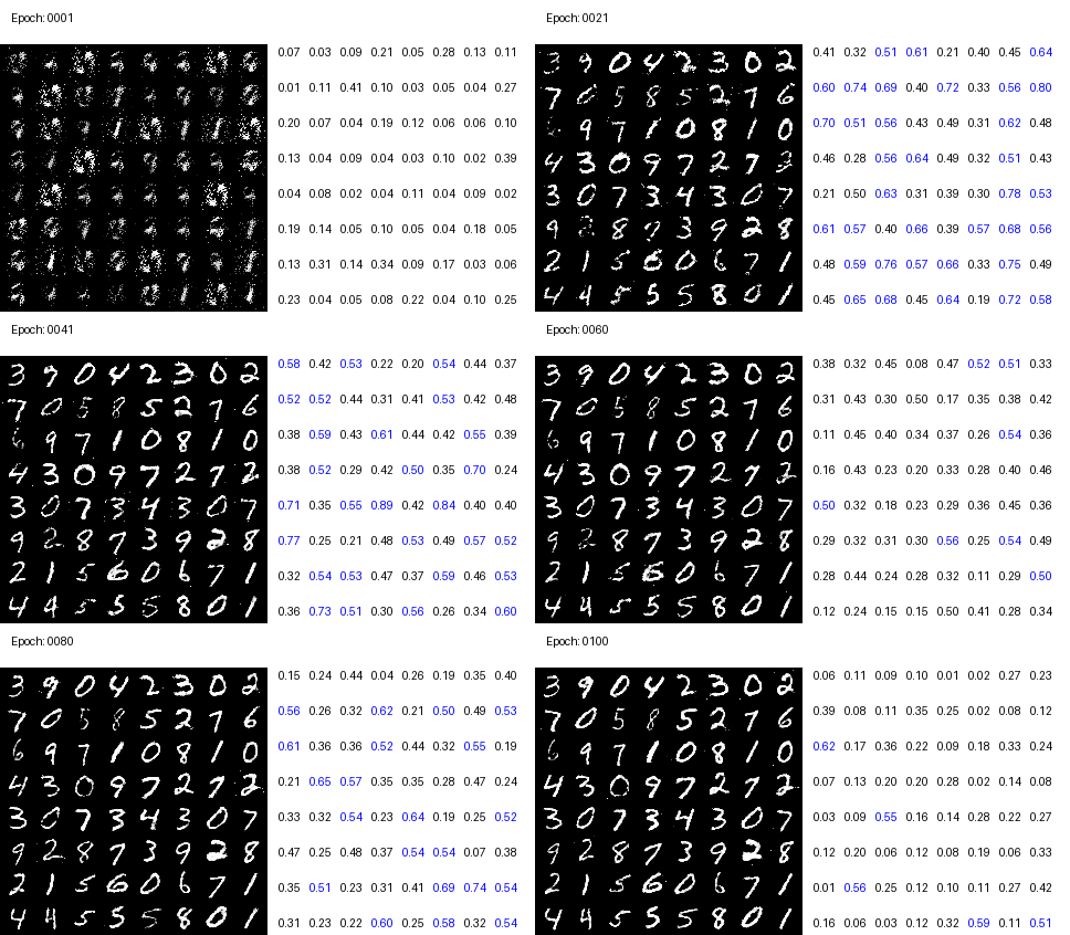

CGAN Generated images and discriminator’s results per epoch (Image by the author)

When examining the generated results, it is evident that the images resemble real digits quite closely. However, the discriminator is much stricter in its scoring compared to human perception of digits.

Comparing the results of CGAN with those of Basic GAN highlights the performance differences more clearly.

Comparison of generated image quality between Basic GAN and CGAN (image by the author)

Conclusion

In this article, we implemented a Conditional GAN (CGAN) and explored how it trains and generates images using the MNIST dataset. Unlike Basic GAN, CGAN provides ‘information’ in vector form to both the generator and discriminator about the type of image to generate. This enables the network to learn based on specific conditions rather than purely random noise, allowing it to generate images that meet specific criteria.

The concept and implementation of CGAN are straightforward. However, how you apply the conditional information and the combination of multiple GANs can lead to various applications like CycleGAN and Pix2Pix. Such application GANs demonstrate the potential of CGAN for tasks such as image translation, style transfer, and text-to-image generation, showcasing the flexibility and extensibility of CGAN.

You can implement and test the Conditional GAN practice code below:

[embed][Hands-On] Understanding Codnitional-GAN and Implementation Hugman Sangkeun Jungcolab.research.google.com