In-Memory Computing vs Processor In-Memory

The Memory Wall Problem

For decades, computing performance has largely been defined by Moore’s Law and Dennard scaling — faster processors, smaller transistors, more performance. But as applications like AI, big data analytics, and high-performance computing grew, another bottleneck began to dominate: the memory wall.

Modern CPUs are fast, but data has to constantly shuttle back and forth between the processor and memory. This “data movement” consumes the majority of energy and time, making the processor spend cycles waiting for memory rather than doing useful work.

To break this wall, two memory-centric paradigms emerged: In-Memory Computing (IMC) and Processor-in-Memory (PIM). While they sound similar, they approach the problem from very different angles.

What is In-Memory Computing (IMC)?

In-Memory Computing (also called Compute-in-Memory, CIM) integrates computation inside the memory array itself. Instead of moving data out to a CPU or GPU, the memory performs operations directly using the physical properties of memory cells. Each SRAM cell now can store and compute!

Below is the standard 6 Transistor SRAM cell

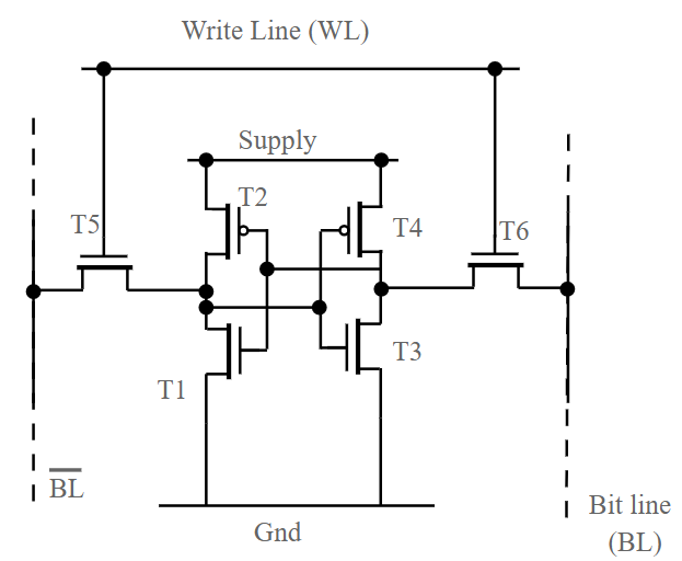
Typical 6 Transistor SRAM cell

Below is the updated SRAM architecture to compute Ternary XNOR. (Used heavily in Binary Neural Networks)

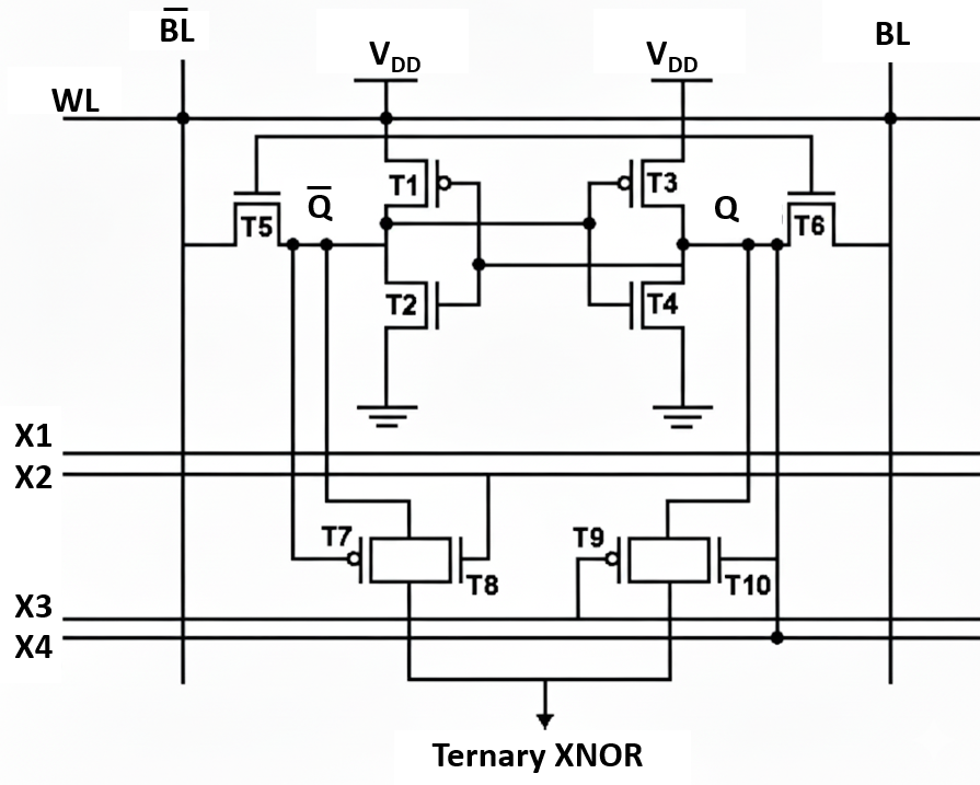
10 Transistor SRAM cell which can compute Ternary NOR

The above architecture is referred from the paper https://ieeexplore.ieee.org/document/10031490

You see, by modifying the SRAM cell architecture, we can now compute Ternary XNOR within the SRAM cell! This eliminates memory access time during inference! By incorporating this design, SRAM block itself can compute on operands before storing data in the cells. The above architecture was designed for Binary Neural networks where XNOR operations are frequently used.

How it works:

• Uses analog operations (e.g., Ohm’s Law in resistive RAM or PCM) or digital logic embedded in SRAM/DRAM arrays.
• Ideal for vector-matrix multiplications, bitwise logic, and neural network inference.

Advantages:

• Massively reduced data movement — compute happens where the data lives.
• Energy efficiency — critical for AI accelerators and edge devices.
• Parallelism — thousands of rows in memory can compute simultaneously.

Challenges:

• Limited flexibility — The above cell can compute XNOR, but not AND!
• Analog noise, precision, and reliability issues.
• Integration with existing memory standards.

What is Processor-in-Memory (PIM)?

Processor-in-Memory (PIM) takes a different route: instead of turning memory into a computational fabric, it places a processor core inside or next to the memory chip. Data computation happens in this processor core, and now memory access time is significantly reduced due to proximity to memory.

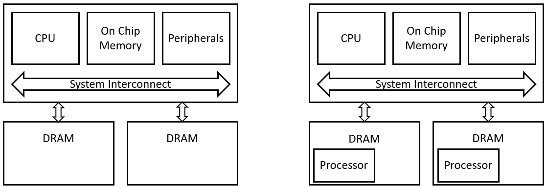
Typical SoC with DDR Memory (Left) vs Modified SoC Architecture incorporating Processor in Memory (Right)

How it works:

• Embeds simple CPUs or specialized accelerators in the same die/package as DRAM.
• These “nearby” processors operate at memory bandwidth speeds, cutting down latency.

Advantages:

• High bandwidth access to memory.
• General-purpose computing possible — processors in memory can run software stacks.
• Less disruptive than full IMC since logic and memory remain logically distinct.

Challenges:

• Fabrication complexity: memory fabs and logic fabs have different process nodes
• Thermal/power management inside dense memory chips.
• Requires new programming models for data and control synchronization between Processor In-Memory and Main system processor.

IMC vs PIM: Head-to-Head

Compute Location

• IMC: Inside memory cells (bit-lines / arrays)
• PIM: Logic cores integrated in or near memory

Operation Type

• IMC: Fixed kernels (e.g., multiply–accumulate, bitwise logic)
• PIM: Programmable cores (general-purpose instructions)

Energy Savings

• IMC: Very high — data never leaves memory
• PIM: Moderate — reduces data movement but doesn’t eliminate it

Precision

• IMC: Limited precision (especially with analog implementations)
• PIM: Full digital precision possible

Flexibility

• IMC: Low (domain-specific accelerators)
• PIM: High (programmable ISA extensions)

Best Use Cases

• IMC: AI inference, pattern matching, associative search
• PIM: Graph analytics, HPC, database queries

Conclusion

Both In-Memory Computing (IMC) and Processor-in-Memory (PIM) aim to tackle the memory wall but from opposite philosophies:

• IMC transforms memory itself into a compute engine.
• PIM integrates processors into the memory system.

The right choice depends on the workload: AI inference loves IMC’s parallelism, while general-purpose data analytics can leverage PIM’s flexibility.