CNN size reduction : Approximating Color Channels and Clustering higher layers.

A technique to compress CNN model using SVD

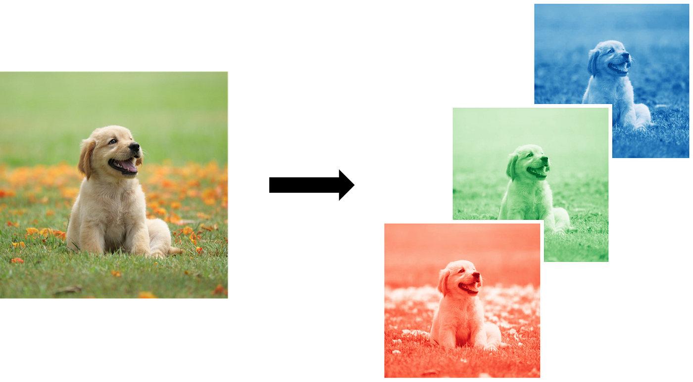
Fig.1 The first layer of the CNN operates on the RGB channel of the input image

The concept is based on the research paper titled as ‘Exploiting Linear Structure Within Convolutional Networks for Efficient Evaluation’.

In this post, I aim to explain the techniques proposed in this paper in a simplified way, translating the theoretical concepts into Python code with a practical example.

Some of the prerequisites,

1. Basic understanding of CNN operations and weight kernels
2. **Low rank approximation of 4D tensors with SVD — refer**

During Training of a convolutional neural network on a particular dataset, the model learns the features of the input image with the help of weight parameters. After the model is trained, it is found that these weight parameters exhibit redundancy. The presence of redundant values increases both the computation operations and the storage space required for the model to be deployed in memory constrained systems.

To address this redundancy in the weight kernels, two different ways of performing approximation have been proposed, which is implemented on an initially trained model.

1. Monochromatic Approximation 2. Bi-clustering Approximation

1. Monochromatic Approximation

It is seen that the weight tensors in the first layer, which involves the color channels from the input feature map lies in the low rank sub-space. That is, even though the weight tensors are in higher dimension, its rank value is lesser as there exists multiple dependent vectors in the weight tensor space. And Hence, it could be approximated by projecting it to 1D subspace without much loss of information.

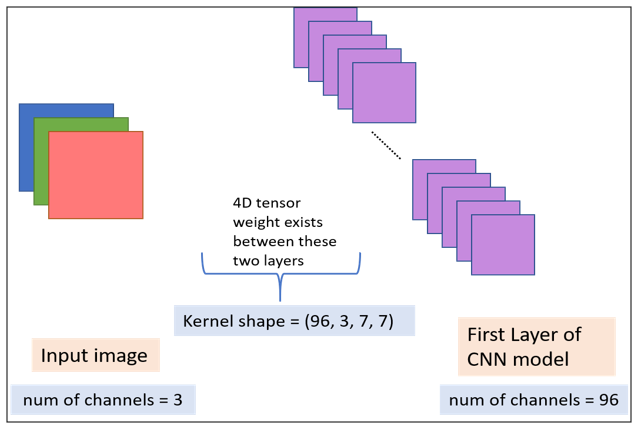
Fig.2 Visualizing kernel weights and feature maps of First Layer in a normal CNN model

In Fig.2, we have visualized the input image channels and the subsequent layer with 96 feature maps. This 96 feature maps have been created by convolving on this 3 input channels with the help of 96 kernel weights, each with dimension (C*k*k)., where C is the number of input channels and k is the spatial dimension of the kernel. The kernel size between these layers can be calculated as 96x3x7x7, which is equivalent to number of output channels, number of input channels, kernel height, kernel width. (bias not considered for simplicity).

Now, we are given the task of reducing this kernel size by projecting it into a lower space. This is done by using a kernel size of (1*1), where the feature map space dimension is reduced as an intermediate step before obtaining the original feature map dimension in the next step.

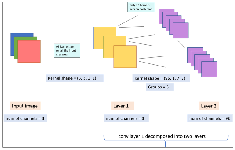
Fig.3 After decomposition, the first layer of the model is divided into two consecutive layers

As seen in Fig.3, The original trained weight tensors are decomposed into two consecutive layers. This decomposition is found to be effective in reducing the number of parameters required for the computation.

Before moving on to How This Decomposition is done, lets take a glance at how the number of parameters have been reduced with the increase in layer count.

The intermediate layer is obtained by using a element-wise operation on the input channel and hence its kernel space is (1*1). A method called clustering is performed between the intermediate and the upper layer. By clustering the intermediate layer (which is the input layer in this operation) and upper layer (which is the output layer), we can tremendously reduce the number of floating point operations performed to obtain the output feature maps.

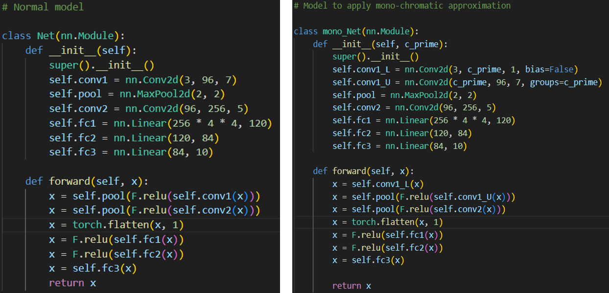
Fig.4 Normal trained CNN model (left) ; First layer decomposed model (right)

Converting a normal CNN model to Monochromatic CNN model

• So, now we train a normal CNN model using our dataset Fig.4 (left).
• We then create a new model with additional layers and extra arguments as seen from the Fig.4 (right).
• This mono-chromatic model uses an additional argument **groups** while creating the convolutional layer. This group argument is responsible for clustering the input and output channels into pre-defined numbers.
• HOW it is Done?.. For group = 3, The following steps happen,

(a) The input and output channels are divided by 3. Therefore, at the Intermediate layer => 3/3 = 1 Upper layer => 96/3 = 32

(b) This means that each of the 32 weight kernels convolve on only 1 intermediate channel to produce 32 output feature maps as shown in Fig.3. So, we obtain three times these output feature map 32 and concatenate it together to produce the final 96 feature maps.

(c) This is completely contrast from the usual convolutional operation where all the 96 weight kernels convolve on all the 3 intermediate channels to produce 96 output feature map.

(d) Total number of parameters in first layer:

Normal model

One layer : (9637*7) [out_channel, in_channel, kernel, kernel]

96x3x7x7 = 14112

Decomposed model

Intermediate layer: (3311) [out_channel, in_channel, kernel, kernel] Upper layer: (96177) [out_channel, in_channel, kernel, kernel]

3x3x1x1 + 96x1x7x7 = 9 + 4704 = 4713

— A reduction of 66.6% in the parameter size of first layer could be achieved.

Now, that we have created the conv-net with decomposed layers, we have to decompose the Original kernel weights to fit these weights into the decomposed weight tensors.

Steps to decompose First layer (color channels) weight kernel

Step 1: Consider Weight dimension of a single kernel

For the model in Fig.4 (left), there are 96 kernels in the first layer each with a size of,

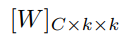
Single kernel size (3D)

Step 2: Fold this into a matrix

To perform SVD approximation, we need to fold the 3-dimension kernel into 2-d matrix. This is done by folding the spatial dimension of the kernel.

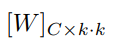
Single kernel folded at spatial dimension (2D)

Step 3: Apply SVD for this matrix with rank=1

For the above weight matrix, SVD is applied and is approximated by considering only the first singular value and vectors.

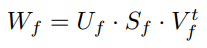
Weight kernel approximated using SVD

Step 4: Repeat step1-step3 for all 96 kernels

The above mentioned step is performed only for a single kernel. We have to perform the operation for all the kernels to approximate them.

Step 5: Find cluster center

We have 96 values of U_f, instead reduce it to 3 values, which corresponds to the number of clusters we are using. This is done by taking mean value of consecutive 32 U_f values. So, each mean value corresponds to the cluster center U_cf.

Python Code for the above mentioned steps

Load the saved state dictionary file and iterate through each kernels in the first layer to perform SVD and save them

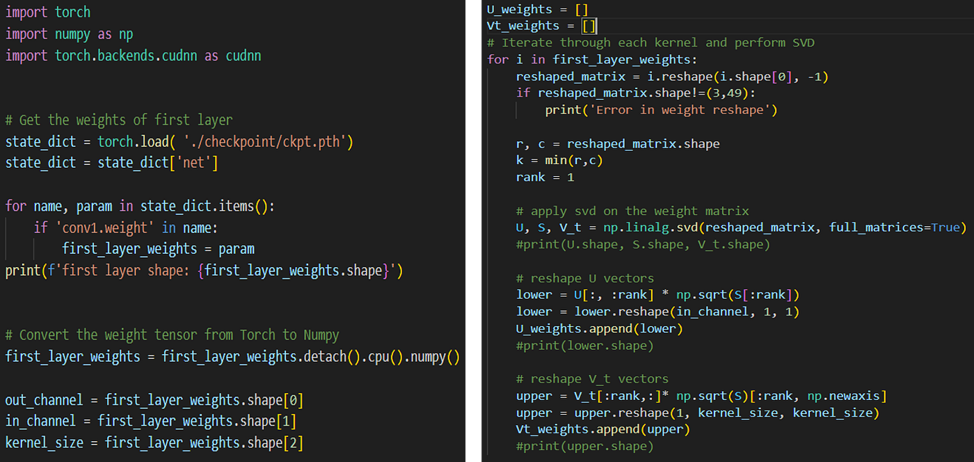
Determine the cluster center of the U-terms and concatenate together to obtain the decomposed weight matrices.

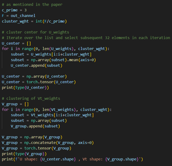
U_shape : 3,3,1,1

Vt_shape : 96,1,7,7

These weights corresponds to the decomposed convolutional layers, which we have created for the monochromatic approximation. Hence, it could be directly fitted onto it.

REFER THE GITHUB CODE FOR WEIGHT TRANSFER DETAILS

Once the weight transfer is done, we fine-tune the monochromatic model to regain its lost performance due to tensor folding and approximations.

2. Biclustering Approximation

In biclustering approximation we cluster the weight kernels of higher convolutional layers and apply low rank approximation techniques on it. Here, both the input and the output channel had to be clustered into equal number of groups. Fig.5 shows how the number of channels and the weight kernel size of a normal CNN model before biclustering operation.

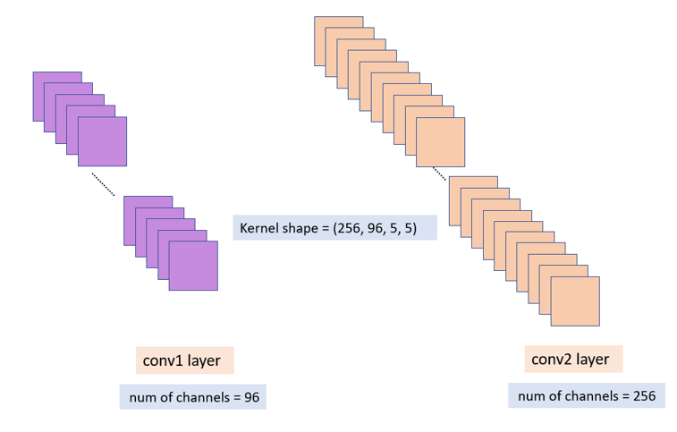
Fig.5 Visualizing the kernel shape of higher convolutional layers

The weight kernel between conv1 layer and conv2 layer can be decomposed by clustering the weight tensor into equal number of groups and perform low rank approximation such as SVD for each of these groups separately.

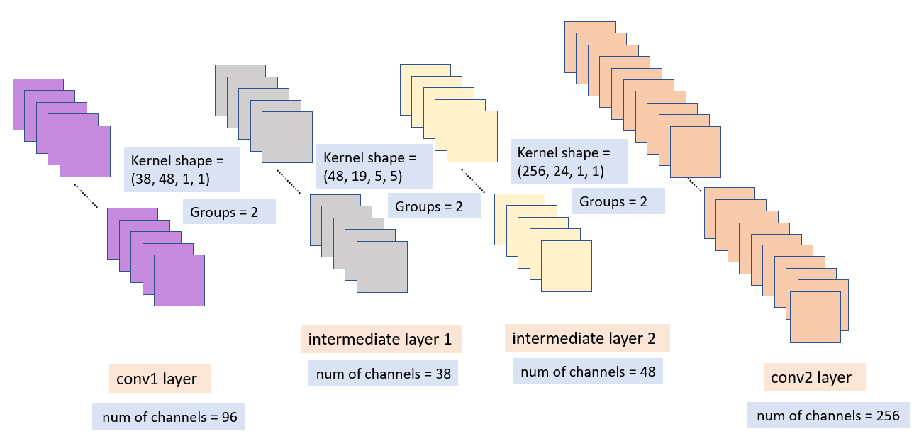
Fig.6 Biclustering approximation of the weight kernel

Steps involved in Bicluster approximation

Step 1: Create a bicluster model

During monochromatic approximation, we have converted our normal model into a monochromatic model that can accommodate the decomposed weights. Likewise, from our monochromatic model we have to update our model to accommodate the decomposed weights obtained after biclustering approximation as seen in Fig.7 (right).

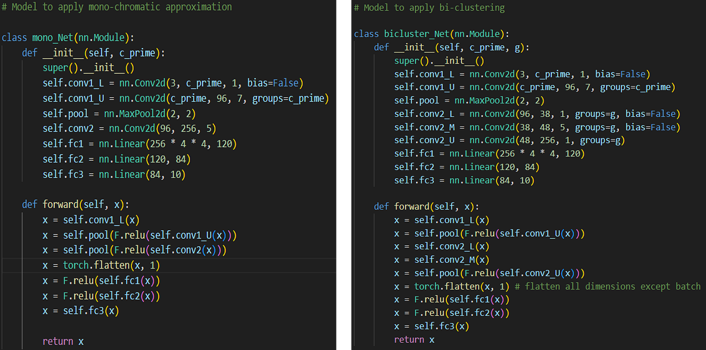
Fig.7 Monochromatic trained CNN model (left) ; Second layer decomposed model (right)

Step 2: Decompose weight kernel

(a) Fold the tensor

The weight tensor is of dimension,

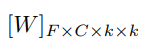
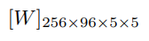
This is folded to get the matrix form, so that we can apply SVD,

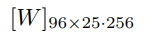
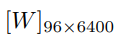
(b) Bicluster and apply SVD

We have divide this weight kernel into two equal parts and apply SVD for both these matrices.

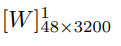
• Perform SVD with k1=19 , and reshape it to 4D tensor

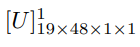
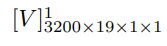
• Square root of the singular value have been combined with the left and right singular vectors.
• The U part is used as the weight tensor for one half of the lower part of the decomposed model.

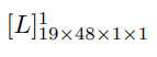
• The V part contains the kernel space and out channel dimension, which is further decomposed by reshaping and applying SVD again with k2=24.

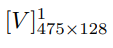
• Second time SVD yields the following weight tensor.

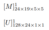
• The weight tensors L1, M1, U1 are composed of one half of the cluster.
• The same set of steps are performed for the other half of the cluster and the results are concatenated.

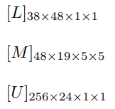
Final approximated weight tensors

• All the above three weight tensors are fitted onto the biclustering model as shown in Fig.7 (right).

Step 3: Check parameter size

Before decomposition : 2569655 = 614400*

After decomposition : 384811 + 481955 + 2562411 = 30768*

Python Code for the above mentioned steps

Load the trained weights from the monochromatic model and access the second layer weights to bicluster and decompose it.

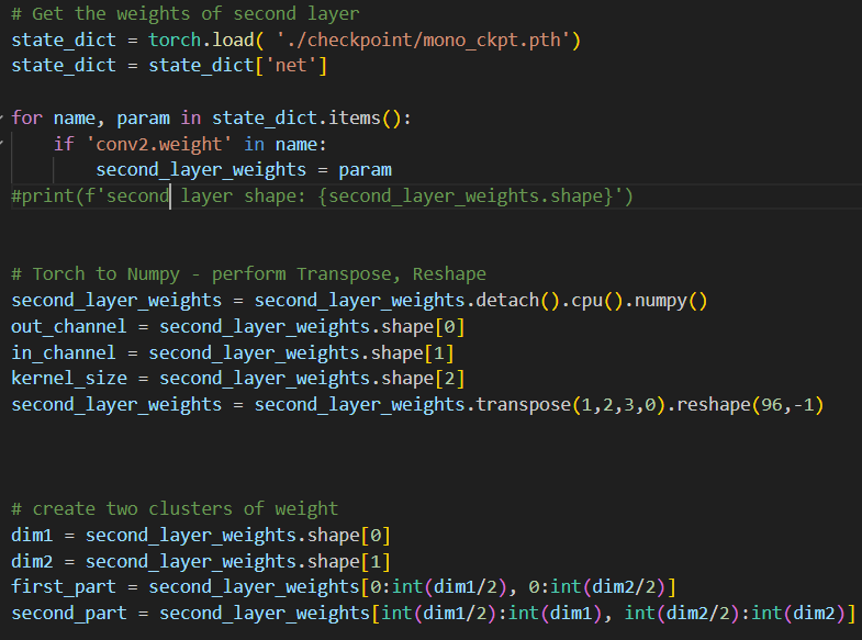
Create a function to repeat the same SVD process for both the clusters.

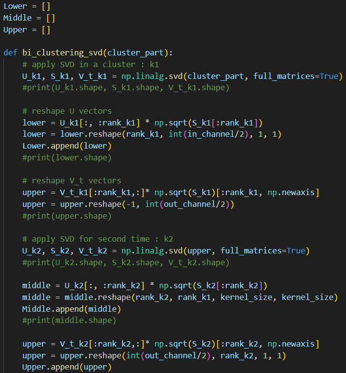
Weight tensors from both these clusters have been concatenated, which is transferred to the model. A normal fine-tuning is performed to regain the lost performance.

concatenate both the cluster to form weight tensor

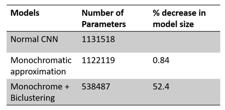
Parameter size after Approximation of kernels

The results are obtained from training a simple CNN model using CIFAR-10 dataset to illustrate the practical implementation of the monochromatic and biclustering approximation techniques. Though the number of convolutional layers increases during this process, the number of parameters in the convolutional layers could be drastically reduced by using this methodology. Further, the redundancy in the fully connected layers can also be approximated using SVD, which has been explained in detail in **my previous blog post.**

GitHub repository : Monochromatic and Biclustering approximation

References

1. Research paper
2. Training Criteria