The Hidden DC Motor Inside Every EV: How Field-Oriented Control Makes a PMSM Behave Like Something Much Simpler

There’s a quiet piece of mathematical sleight-of-hand running inside every modern electric vehicle, every CNC machine, every industrial robot — and most engineers who work adjacent to these systems have never seen it spelled out clearly.

Your EV’s traction motor is a three-phase AC machine. The currents flowing into it are sinusoids. The rotor flux rotates. Everything is time-varying, coupled, and nonlinear.

But the software controlling it thinks it’s talking to a DC motor.

That’s not an approximation. It’s a coordinate transform — and once you see it, the entire architecture of a modern servo drive snaps into focus.

Why DC Motors Are So Easy to Control

Before we unroll the trick, we need to understand why anyone would want a DC motor in the first place.

A brushed DC motor is described by two equations. The electrical side:

Vₐ = Rₐiₐ + Lₐ(diₐ/dt) + Kφω

And the mechanical side:

J(dω/dt) = Tₑ — T_L — Bω

The electromagnetic torque is simply:

Tₑ = Kφ · iₐ

That last equation is the key. Torque is proportional to a single current. Want more torque? Increase iₐ. The proportionality constant Kφ is fixed by the machine geometry. There’s no coupling between axes, no rotating quantities, no trigonometry in your control loop.

A PI controller on iₐ gives you direct, linear, instantaneous torque control. This is why brushed DC drives dominated industry for decades — the control problem is simple.

The problem? Brushes. They wear out. They spark. They cap your maximum speed. They generate EMI. For anything demanding — EV traction, semiconductor manufacturing equipment, precision CNC — they’re a non-starter.

The Permanent Magnet Synchronous Motor (PMSM) solves all of that. No brushes, no commutator, high efficiency, compact and lightweight. But it comes with a much harder control problem.

The PMSM: Powerful, Efficient, and a Control Nightmare

A PMSM has three-phase stator windings fed with three-phase AC. The rotor carries permanent magnets. When the stator currents are sequenced correctly, they produce a rotating magnetic field, and the rotor’s permanent magnets lock onto it and get dragged along — that’s synchronous operation.

The three-phase currents look like this:

iₐ = Im·cos(ωₑt) i_b = Im·cos(ωₑt − 120°) i_c = Im·cos(ωₑt − 240°)

Now try writing a torque controller in terms of these. The torque involves products of sinusoids, rotor position, and magnetic flux. You cannot stick a PI controller on a sinusoid and expect zero steady-state error — the integrator sees a signal that never settles.

The full voltage equations in the natural abc frame are ugly. The d and q axes couple through speed-dependent terms. A voltage command on one axis disturbs the other. It’s a nonlinear, multi-input multi-output system.

The solution is to stop fighting the rotating frame and instead join it.

The Clarke Transform: From Three Phases to Two

The first step is to reduce the three-phase system to an equivalent two-phase system. Three balanced sinusoids contain redundant information — the third phase is always minus the sum of the other two. The Clarke transform projects abc onto two orthogonal axes (α and β) in a stationary frame:

iα = iₐ iβ = (1/√3)(iₐ + 2i_b)

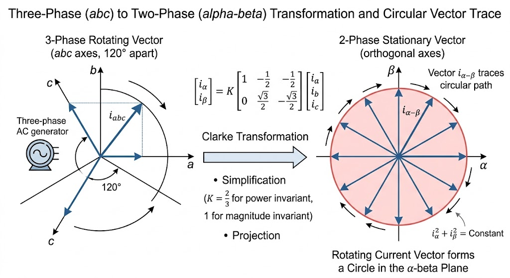
The result is a two-dimensional vector rotating at ωₑ in the stationary αβ frame. The current is still sinusoidal — we haven’t eliminated the rotation yet. But we’ve reduced complexity from three variables to two.

The Park Transform: The Core Idea

Here is the central insight. If you have a vector rotating at ωₑ, and you look at it from a coordinate frame that also rotates at ωₑ — the vector appears stationary.

Think of it this way: imagine you’re sitting on the rotor, spinning with it. From your seat, the rotor magnets aren’t moving at all — they’re just sitting there, pointing in a fixed direction. The stator currents, which from the outside look like a rotating wave, now look like a steady push in a fixed direction. You’ve turned a time-varying sinusoidal problem into a static one, simply by changing where you’re standing.

This is exactly what the Park transform does. It rotates the αβ axes at the electrical frequency ωₑ, tracking the rotor flux angle θₑ in real time:

id = iα·cos(θₑ) + iβ·sin(θₑ) iq = −iα·sin(θₑ) + iβ·cos(θₑ)

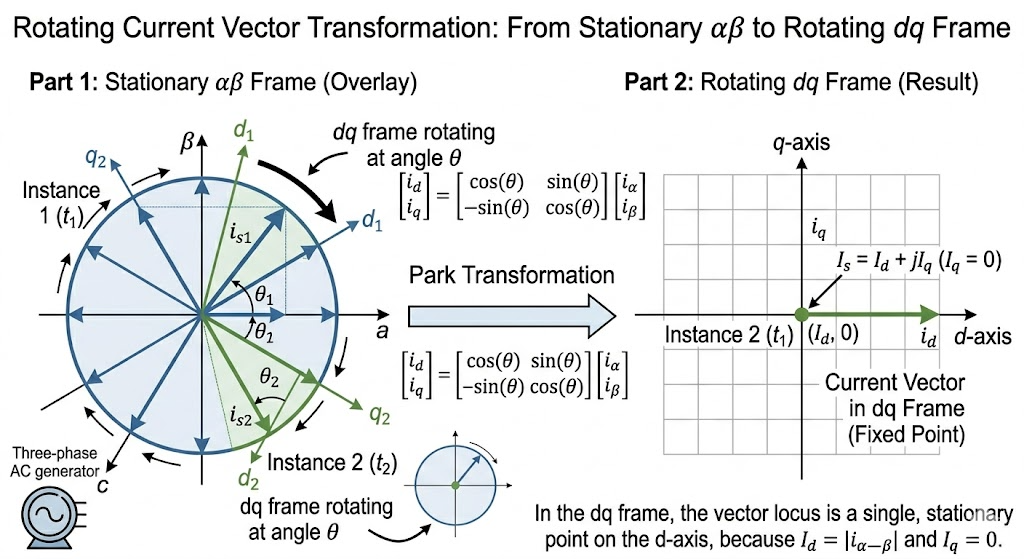
Substituting the sinusoidal expressions for iα and iβ and using θₑ = ωₑt:

id = Im·cos(φ) ← constant iq = −Im·sin(φ) ← constant

The sinusoidal three-phase currents have become DC values. That’s it. That’s the whole trick.

The combined Clarke + Park transform written as a single matrix is:

[id] = (2/3) · [cos θₑ cos(θₑ−120°) cos(θₑ−240°) ] · [iₐ] [iq] [−sin θₑ −sin(θₑ−120°) −sin(θₑ−240°)] [i_b] [i_c]

The 2/3 factor is a normalization choice — the amplitude-invariant convention, standard in motor drives.

What the dq Frame Gives You

In the rotating dq frame, the PMSM voltage equations become:

Vd = Rs·id + Ld(did/dt) − ωₑ·Lq·iq Vq = Rs·iq + Lq(diq/dt) + ωₑ·Ld·id + ωₑ·λpm

And the electromagnetic torque works out to:

Tₑ = (3/2)·p·[λpm·iq + (Ld − Lq)·id·iq]

For a surface-mounted PMSM (SPM) where Ld = Lq, the reluctance term vanishes:

Tₑ = (3/2)·p·λpm·iq

Compare this with the DC motor result:

Tₑ = Kφ · iₐ

They are structurally identical. λpm is fixed (permanent magnet), p is fixed (pole count geometry). Torque is proportional to iq alone.

Set id = 0, control iq, and the PMSM behaves like a separately-excited DC motor — with all the efficiency and reliability advantages of an AC machine. This is the core insight of Field-Oriented Control.

Where the Cross-Coupling Terms Come From

Look again at the voltage equations. Even in the dq frame, the axes are not fully decoupled:

−ωₑ·Lq·iq — the q-axis current bleeds into the d-axis voltage. The faster the motor spins (higher ωₑ) and the more torque current you push (higher iq), the worse this gets.

+ωₑ·Ld·id — symmetric in the other direction. The d-axis flux current disturbs the q-axis.

ωₑ·λpm — the back-EMF from the permanent magnet, which grows linearly with speed and acts as a disturbance on the q-axis.

These cross-coupling terms are what make the system nonlinear. In Field-Oriented Control current loops, they are cancelled by feedforward decoupling — the controller adds these terms explicitly as feed-forward compensation, so each axis sees a clean, independent first-order system. This is what allows two separate PI controllers (one for id, one for iq) to work well in practice.

The Cascade Control Architecture

Now that torque reduces to controlling iq, the full servo drive implements three nested control loops, each running at a different sample rate:

Current loop (innermost, fastest — ~16 to 64 kHz) Regulates id and iq to their references. Two PI controllers, one per axis, with feedforward decoupling:

Vq = PI_q(iq − iq) + ωₑ·Ld·id + ωₑ·λpm Vd = PI_d(id − id) − ωₑ·Lq·iq

This loop must be fast because it sits inside everything else. Its bandwidth (~1–5 kHz) sets the ceiling for the loops above it.

Velocity loop (middle — ~4 kHz) Takes speed reference ω, measures actual speed from the encoder, outputs iq. A PI controller. The speed estimate from the encoder is differentiated position, which gets noisy at low speed — a tracking observer or low-pass filter smooths it, but that filter adds phase lag and limits bandwidth. This is the classic tradeoff in velocity control.

Position loop (outermost, slowest — ~1 kHz) Takes position reference θ, outputs velocity reference ω. Typically a pure P controller — integral action in the position loop causes windup and overshoot. Feedforward from the trajectory profile dramatically reduces following error during motion.

Each inner loop must be 5–10× faster than the outer loop. This is not a rule of thumb — it’s the mathematical condition under which the inner loop appears as unity gain to the outer loop, letting you design each loop independently.

The Hardware That Makes FOC Real

Field-Oriented Control is an elegant theory. Making it work in practice requires three hardware subsystems that are often underappreciated.

The Inverter

The inverter converts a DC bus voltage (typically 560V from a 400V three-phase supply) into the variable three-phase voltages the motor needs. Six power switches — arranged as three half-bridges — are switched by Space Vector PWM (SVPWM) at 8–100 kHz depending on the switch technology.

Modern drives are moving from IGBTs to Silicon Carbide (SiC) MOSFETs. The reason is physics: silicon’s on-resistance scales as V_BR².5, meaning a 600V silicon switch has roughly 10× higher conduction losses than a 100V device of the same die area. SiC’s wider bandgap breaks this relationship, enabling low conduction loss and fast switching at 600–1700V simultaneously. The result: SiC drives run at 50–200 kHz switching frequency with lower total losses than IGBTs at 10 kHz — better current waveforms, smaller filters, higher control bandwidth.

The Encoder

FOC requires the rotor angle θₑ in real time. Every Park and inverse-Park transform depends on it. The encoder is therefore not optional instrumentation — it is in the inner loop of the fastest control path in the system.

High-performance servo drives use optical sin/cos encoders: instead of digital pulses, they output analog sin(θ) and cos(θ), which the drive interpolates into millions of counts per revolution. An encoder with 2048 lines and 2048× interpolation gives roughly 4 million counts per revolution — nanometre-level positioning when the mechanical geometry is right. Resolution and latency here directly set the maximum achievable control bandwidth above.

Current Sensing and ADC Timing

The current loop runs at up to 64 kHz. Phase currents must be sampled, Park-transformed, and fed to two PI controllers within a single PWM period (~15 µs at 64 kHz). This is the most accuracy-critical measurement in the drive.

The subtlety most textbooks skip: you cannot sample the current at an arbitrary point in the PWM cycle. The phase current has the fundamental component you want plus switching ripple at the PWM frequency superimposed on top. Sample at the wrong moment and you measure fundamental + ripple. The solution is synchronised sampling — the ADC is triggered at the PWM carrier peak or valley, exactly where the ripple averages to zero.

Even a correct sensor placement fails if the two phase currents are not sampled simultaneously. A time difference between sampling iₐ and i_b means the Park transform operates on currents from different instants — that phase error shows up as torque ripple. High-performance drives use simultaneous-sampling ADC pairs or sample-and-hold circuits ahead of a single converter.

Putting It All Together: Signal Flow in a Servo Drive

Here is the complete signal chain, from trajectory command to motor current:

Every block in that diagram exists for a reason that traces back to the original problem: sinusoids are hard to control, DC is easy, and the Park transform is the bridge between them.

Why This Matters Beyond EVs

The same architecture runs in:

• EV traction drives — Tesla, BMW, every modern electric powertrain. The PMSM’s high power density and the wide field-weakening range above base speed (constant power region) make it ideal for traction.
• Industrial servo drives — Robot joints, CNC axes, pick-and-place machines. Sub-millisecond torque response, nanometre-level position control.
• Wind turbine generators — PMSMs used as generators, FOC running in reverse (controlling generator torque to track the MPPT operating point).
• Linear motors in semiconductor fabs — ASML’s wafer stages use planar linear synchronous motors. The dq model transfers directly from rotary to linear (replace pole pairs p with π/τ where τ is the pole pitch). Sub-nanometre positioning at metre-per-second velocities. The most demanding motion control application in existence.

The One-Sentence Summary

A PMSM is a rotating AC machine. The Park transform converts it into a stationary DC machine in a spinning frame of reference. FOC controls that DC equivalent with two PI loops, then transforms the result back into three-phase voltages. Everything else — the inverter, the encoder, the ADC timing, the gate drivers — exists to make that transform work in real time, at high power, without killing anyone.

That’s the hidden DC motor inside your EV.