YoloV2 Object detection Model

YoloV2

Purpose: YOLOv2 performs real-time object detection, predicting bounding boxes and class probabilities directly from an input image in a single pass.

Problem Statement: Efficiently detect and classify objects in images while balancing speed and accuracy.

what kind of model is YOLOV2?

YOLOv2 is a single-stage object detection model.

let’s define what is single stage and multistage object detection model

Single-stage detection: Detects objects in one pass by directly predicting bounding boxes and class probabilities (e.g., YOLO, SSD). Faster but slightly less accurate.

Multi-stage detection: Performs detection in multiple steps, like generating region proposals first, then refining and classifying them (e.g., Faster R-CNN). More accurate but slower.

let’s discuss how yolov2 works:

1. Input Image:

• YOLOv2 accepts images resized to a fixed size of 416x416 pixels.
• This resizing ensures that all images processed by the network have a uniform size, allowing for efficient batch processing.
• The image is normalized (pixel values scaled between 0 and 1) for faster convergence during training.

2. Convolutional Layers:

• YOLOv2 uses Darknet-19 as its backbone, a lightweight and efficient convolutional neural network.
• It consists of 19 convolutional layers followed by 5 max-pooling layers.
• These layers extract spatial and semantic features from the input image, enabling the detection of objects at various scales.
• Batch normalization is applied after each convolution to stabilize training and improve generalization.

3. Grid Division:

• The input image is divided into a grid of 13x13 cells.
• Each cell is responsible for predicting objects whose center falls inside that cell.
• This grid-based division enables the model to perform object localization by predicting bounding boxes relative to the grid cell coordinates.

4. Anchor Boxes:

• Anchor boxes are predefined bounding box templates with various aspect ratios and sizes.
• Each grid cell predicts bounding boxes by adjusting these anchor boxes.
• YOLOv2 uses 5 anchor boxes per grid cell, enabling it to detect objects of different shapes and sizes.
• The use of anchor boxes solves YOLOv1’s issue of struggling with multi-object detection when objects have varying sizes.

5. Bounding Box Prediction:

• Each grid cell predicts 5 bounding boxes, and for each box, it outputs:

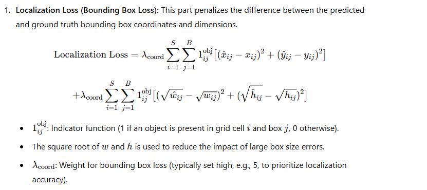
1. x, y: The center coordinates of the box (relative to the grid cell).
2. w, h: The width and height (adjusted relative to the anchor box).
3. Confidence score: Probability of the box containing an object.

• This confidence score is a product of the objectness score (is there an object in the box?) and the Intersection over Union (IoU) between the predicted box and the ground truth.

6. Class Prediction:

• Each grid cell predicts the class probabilities for the object it detects.
• For example, if there are 20 classes (e.g., VOC dataset), the model outputs a 20-dimensional vector of probabilities for each grid cell.
• The final output for each grid cell combines the confidence scores of bounding boxes and class probabilities to determine the object type and location.

7. Non-Maximum Suppression (NMS):

• After predictions, there are often multiple bounding boxes for the same object.
• NMS removes redundant bounding boxes by keeping only the box with the highest confidence score while discarding others with overlapping IoU > a threshold (e.g., 0.5).
• This step ensures that only the most relevant bounding box is retained for each detected object.

Difference between yolov1 and yolv2:

Pros of YOLOv2:

1. Fast Detection:

• Achieves real-time object detection with a balance of speed and accuracy, making it suitable for applications like video processing and autonomous systems.

2. Improved Accuracy:

• Introduced anchor boxes, batch normalization, and a better backbone (Darknet-19), resulting in higher mean Average Precision (mAP) compared to YOLOv1.

3. Multi-Scale Detection:

• Uses multi-scale training, enabling the model to detect objects at various sizes and scales effectively.

4. End-to-End Training:

• YOLOv2 is a single-stage detector, meaning it combines feature extraction, classification, and localization into one streamlined process, simplifying training and inference.

5. Compact Model:

• Darknet-19 is a lightweight and efficient backbone, making YOLOv2 deployable on devices with limited computational resources.

6. Generalized Detection:

• Performs well across different datasets due to k-means clustering on bounding boxes and multi-scale training.

Cons of YOLOv2:

1. Struggles with Small Objects:

• While YOLOv2 improves over YOLOv1, it still has difficulty detecting very small objects due to down sampling in the network.

2. Less Accurate Than Two-Stage Detectors:

• Compared to two-stage detectors like Faster R-CNN, YOLOv2 sacrifices some accuracy for speed, making it less suitable for applications requiring high precision.

3. Overlapping Objects:

• YOLOv2 can struggle with detecting overlapping objects in close proximity because each grid cell can only predict a limited number of bounding boxes.

4. Dependence on Anchor Boxes:

• Performance is highly dependent on well-chosen anchor box sizes and aspect ratios, which require tuning for specific datasets.

5. High Computational Cost for Small Objects:

• Detecting small objects effectively requires a finer grid size, increasing computational overhead.

Limitations of YOLOv2:

1. Grid Cell Constraint:

• Each grid cell is responsible for detecting one object, which can lead to errors when multiple small objects fall within the same cell.

2. Fixed Aspect Ratios:

• The predefined anchor box aspect ratios may not generalize well to datasets with unusual object shapes, requiring manual adjustment.

3. No Instance Segmentation:

• YOLOv2 focuses on bounding box detection but does not support tasks like instance segmentation.

4. Limited Context Awareness:

• YOLOv2 operates at a fixed grid size and can miss contextual details in complex scenes compared to more advanced detectors.

5. Scaling Issues for Complex Datasets:

• On datasets with highly complex object distributions (e.g., COCO), YOLOv2 struggles to match the accuracy of newer architectures like YOLOv3 or YOLOv4.

1. anchor boxes and fine-tuned their sizes using k-means clustering?
2. multi-scale training and how it improves YOLOv2’s robustness?

1. Anchor Boxes and Fine-Tuned Their Sizes Using K-Means Clustering

Anchor boxes are predefined bounding box shapes and sizes used to detect objects of different aspect ratios and scales. YOLOv2 refines the choice of anchor boxes using k-means clustering on the training dataset.

How K-Means Clustering Works for Anchor Boxes:

1. Purpose:

• Instead of manually defining anchor box dimensions, k-means clustering ensures the sizes of anchor boxes match the ground truth bounding boxes in the dataset.

2. Process:

• Compute the aspect ratio and size of each ground truth bounding box in the training dataset.
• Apply k-means clustering to group these bounding boxes into k clusters (e.g., 5 clusters in YOLOv2).
• The centroids of the clusters represent the optimal anchor box sizes.

3. IoU Distance Metric:

• Standard k-means clustering uses Euclidean distance. However, YOLOv2 uses the IoU (Intersection over Union) metric to determine how well an anchor box matches a bounding box: IoU Distance=1−IoU between ground truth and anchor box\text{IoU Distance} = 1 — \text{IoU between ground truth and anchor box}IoU Distance=1−IoU between ground truth and anchor box

4. Benefits:

• Ensures anchor boxes are tailored to the dataset, improving object detection accuracy.
• Reduces localization errors, especially for objects with unusual aspect ratios or sizes.

2. Multi-Scale Training and How It Improves YOLOv2’s Robustness

Multi-scale training is a technique in YOLOv2 where the model is trained on input images of varying resolutions, improving its ability to detect objects across different scales and sizes.

How Multi-Scale Training Works:

1. Random Resizing During Training:

• During training, the input image resolution is randomly resized every few batches. For example:
• Sizes: 320×320,352×352,…,608×608
• Resolutions are multiples of 32, aligning with the network’s stride.
• The network must adapt to different input sizes, making it robust to scale variations.

2. Adjusting the Grid Size:

• The grid size (e.g., 13×13) changes with the input resolution.
• Larger input sizes provide finer grid cells for detecting small objects, while smaller input sizes improve detection speed.

3. Inference Flexibility:

• After multi-scale training, the model can process images of varying resolutions during inference without significant performance degradation.

Benefits of Multi-Scale Training:

1. Robustness:

• Makes YOLOv2 more resilient to objects of varying sizes and resolutions.

2. Better Small Object Detection:

• Higher resolutions enable the model to detect smaller objects by generating finer grid cells.

3. Generalization:

• Improves generalization across datasets with different image resolutions.

Example:

• Suppose a model trained only on 416×416 images may fail to detect objects in high-resolution images (e.g., 608×608).
• Multi-scale training ensures the model can seamlessly handle both low and high-resolution images.