Build a GAN (part 1)

I will start with some points and reminders that are needed to understand this article

• Convolutions:

if you are not very familiar with convolutions, here is a quick reminder:

torch.nn.Conv2d(in_channels, out_channels, kernel_size, ..)

in_channels in the number of channels of the input tensor (ex 3 if it is an RGB image)

• Batch Normalization :

When the weights of a layer are too large, it causes problems because a tiny change in the input results in a massive change in the output (and intuitively, this phenomenon is not “natural”). Large weights are also not very compatible with activation functions like tanh and sigmoid.

Batch Normalization solves this. It also addresses Internal Covariate Shift. It makes sure every layer receives input in a reasonable interval. The Batch Normalization is a layer on its own and it has two learnable parameters that will help to normalize the data.

• Weights initialization:

To avoid large weights, one can also initialize the weights around 0, for example we can use “He initialization”, so for a layer containing n parameters, weights are drawn from a normal distribution: ~ N(0, √(2/n)) . (here n is depends on the number of parameters of the layer)

Most GAN explanatory articles online use a lot of theory. In contrast, in this article we will see GANs like a machine, and when you build a machine, you don’t really focus on what mathematical model the machine represents, or the ideal machine according to theory, etc. You just build the machine and then experiment and try various modifications until something works. We will only use theory if it is essential to understand something.

So our goal is to generate fake realistic faces.

The big picture of a GAN is as follows:

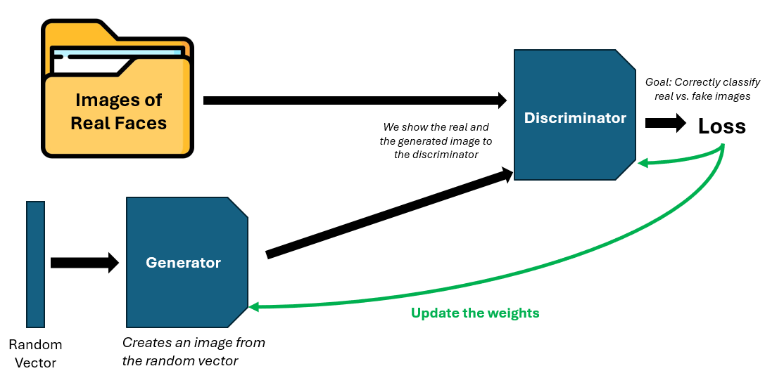
For the Discriminator, we minimize the number of incorrect guesses. It’s a binary classification task: real faces are 1 and fakes are 0. The Discriminator should correctly classify both. If we present a fake face and it is classified as 0, it is good for the Discriminator but bad for the Generator. Conversely, if a fake face is classified as 1, it is bad for the Discriminator but good for the Generator

The training process involves two distinct parts of the loss function:

• Loss on real images: When we present a real face x, we want the discriminator to classify it as real (output close to 1). Therefore, we update the discriminator to minimize the loss −log(D(x))
• Loss on generated images: When we present a fake face, y ,there is a conflict. The discriminator wants to classify it as fake (output close to 0), so it tries to minimize −log(1−D(y)). The generator, however, wants to trick the discriminator. To do this, we update the generator weights to minimize the opposite loss: −log(D(y))

So to train the GAN, we take a real image x and a fake image y . First, we look at the Discriminator: we calculate the total discriminator loss, −log(D(x))−log(1−D(y)) , and use the gradients to update its weights. Next, we look at the Generator: we calculate its specific loss, −log(D(y)) , and use those gradients to update the generator’s weights.

a pseudo code would look like :

for each epoch:
    for each real_image in real_images:
        fake_image = generate_fake()
        #Update Discriminator
        loss_D = -log(D(real_image)) - log(1 - D(fake_image))
        Update D weights to minimize loss_D

        #Update Generator
        fake_image = generate_fake()  
        loss_G = -log(D(fake_image))
        Update G weights to minimize loss_G

(we can also generate fake_images only once, it is totally fine, but i prefer to show the algorithm of the original GAN paper) Of course in reality we don’t iterate through real images one by one, but we use batches like this:

for epoch in range(num_epochs):
    for real_images in dataloader:
        #Train Discriminator 
        fake_images = generate_batch_of_fakes()

        loss_D = -torch.log(D(real_images)).mean() - torch.log(1 - D(fake_images)).mean()
        D_optimizer.zero_grad()
        loss_D.backward()
        D_optimizer.step()

        #Train Generator
        fake_images = generate_batch_of_fakes()
        loss_G = -torch.log(D(fake_images)).mean()
        G_optimizer.zero_grad()
        loss_G.backward()
        G_optimizer.step()

So to train a GAN to generated we need training data.

I downloaded this dataset of faces : https://www.kaggle.com/datasets/ashwingupta3012/human-faces?resource=download . I processed the images to make each image have a size of 64×64×3, and currently, we have around 7,000 images of real faces. This is not a big dataset at all, and we could probably get better results if we used another dataset, but let’s just stick with that one and see if we can do something with it.

a sample of the dataset :

Now, when we run that training loop, when do we know we need to stop the training? This is a good question, because it is impossible to have very low loss on both the discriminator and the generator we are training. If we have a very good discriminator, it means that our generator is not that good, and vice versa.

In theory, we need to stop when the quality of the generated images is good. Also, increasing the number of epochs does not necessarily lead to better results.

We will begin our experimentation with a simple generator/discriminator (with only linear layers)

images generated with a very simple GAN

The results are not good at all. We need to make some adjustments.

I tried to use a simple discriminator and a convolutional generator, and I also tried to use a simple generator (linear layers) and a more complex discriminator (with convolutional layers). As you can see:

The discriminator gets better faster than the generator. And this is a problem because it will be very difficult for the generator to trick the discriminator. Intuitively, if the discriminator gets almost all its answers correct, it will be very difficult for the generator to know what is “correct” and what is “wrong” in the generation. (Explanation with gradients: because a small discriminator loss means the generator loss -log(D(y)) will be very large: +inf and so D(y) is near 0. This puts it in the flat part of the sigmoid, so the gradient ∂-log(D(G_θ(z))/∂θ will be very very small.

gradient of the generator :

σ is the same as the discriminator (it is a sigmoid). a is some activation output

and :

is very small when σ(a) is ≈ 0 or ≈ 1.

If the generator gets better faster than the discriminator, it means the generator learned to trick the discriminator. It generates an image that the discriminator always accepts as a face, making it difficult for the discriminator to find the right path back.

In a perfect scenario, we need to train until both the discriminator and generator get stuck with a loss of 0.6931 for a long time. Ideally, at the end, the generator’s distribution equals the real data distribution, so the best the discriminator can do is output 0.5 every time.

Outputting 0.5 for everything corresponds to a loss of 0.6931. But the important bit isn’t the value; it’s that neither network can reduce its own loss anymore given the other is fixed. That’s exactly a Nash equilibrium. Don’t forget that what makes learning happen is the gradient, not the absolute loss value.

Maybe we got bad results because we didn’t pick the right learning rate or mini-batch size? The hyperparameter space is vast, so we will use Grid Search and Random Search to find some valid combinations, and then I will inspect the visual results.

After trying many hyperparameters, there isn’t a combination that really stands out or produces realistic faces…

some generated faces after using grid search

..So, we need to dig deeper to find solutions. We noticed that the discriminator has an easier task (especially at the beginning): It is much easier to distinguish between a real and a fake image than to generate images from scratch.

Generating an image is difficult: most pixel combinations are just noise, and the truly realistic combinations that produce images of faces are rare. So, I tried to modify the learning rate dynamically depending on the generator loss, but the results were not good..

Another thing I observed is that having a high generator loss and a high discriminator loss doesn’t necessarily mean that our model isn’t doing well.

Sometimes the generator produces the same image every time. To fix this, I think we need to avoid bias in the weights, or simply avoid tiny weights or activations that are equal to zero in the generator. This is because very small weights mean we almost cancel all previous layers and start fresh with the bias term, so the output will no longer depend on the random latent vector. Batch normalization can help avoid having very small weights. Also, we almost always use LeakyReLU, and that’s good because it prevents activations equal to zero.

The loss curve can have many optimal minima, and I have the intuition that there are two types: strict local minima (which produce an image that tricks the discriminator) and more gradual minima (which are images of real faces). But to confirm this, we need a better visualization of the loss function (perhaps in part 2 of this article).

The problem is that the goal of the generator is not to produce a face, but to produce a photo that can be classified as coming from the same set of real photos by the discriminator. And okay, you might think that the common attribute is having a realistic face, but I can tell you the commonality might just be ‘a valid eye’ or a valid ‘nose.’ So, maybe the generator will produce photos of flawed faces that happen to have valid eyes, and they will be considered valid by the discriminator.

The generator sometimes learns to trick the discriminator rather than generate realistic images. I tried several approaches to fix this: gradually increasing discriminator complexity every 10 epochs, switching discriminators every n epochs, and alternating fresh discriminators each epoch with warm-up training. None worked. When we try with a new discriminator, it is not initially good, so the generator learns nothing. However, when I warmed up the discriminator a bit before using it, it caused the discriminator to overfit on the training data. This led the generator to exploit specific pixel patterns that fool the discriminator without producing actual faces.

Let’s look at the literature a bit to find what we’ve done wrong...let’s first look at DCGAN .

First, they use a CNN for both the generator and the discriminator. In this CNN, they don’t use pooling layers because pooling layers apply a fixed rule (e.g., selecting the maximum value in small windows like 2×2) with no learnable parameters. Instead of these fixed rules, they use basic convolutional layers with strides larger than one pixel (e.g., stride = 2).

Second, they don’t use the fully connected layers we usually see at the end of a CNN. Third, they apply batch normalization on almost all layers. Fourth, they use the ReLU activation function for the generator with a tanh function for the output. For the discriminator, they use leaky ReLU.

They use a mini-batch size of 128 and initialize weights from a normal distribution N(0, 0.02).

At the beginning, they tried to generate photos of bedrooms, making sure that during training, the model sees each image only once (to avoid the model memorizing the real images). They also removed similar-looking images from the training data. To do this, they implemented this system:

So, according to their paper, they use a generator like this :

class Generator(nn.Module):
    def __init__(self, z_dim):
        super(Generator, self).__init__()
        self.main = nn.Sequential(
            # input is Z, going into a convolution
            nn.ConvTranspose2d( z_dim, 64 * 8, 4, 1, 0, bias=False),
            nn.BatchNorm2d(64 * 8),
            nn.ReLU(True),
`
            nn.ConvTranspose2d(64 * 8, 64 * 4, 4, 2, 1, bias=False),
            nn.BatchNorm2d(64 * 4),
            nn.ReLU(True),

            nn.ConvTranspose2d( 64 * 4, 64 * 2, 4, 2, 1, bias=False),
            nn.BatchNorm2d(64 * 2),
            nn.ReLU(True),

            nn.ConvTranspose2d( 64 * 2, 64 , 4, 2, 1, bias=False),
            nn.BatchNorm2d(64),
            nn.ReLU(True),

            #convert back to RGB image
            nn.ConvTranspose2d( 64 , 3 , 4, 2, 1, bias=False),
            nn.Tanh()
        )

    def forward(self, input):
        return self.main(input)

And these hyperparameters: learning rate of 0.0002, Beta1 of 0.5.

They trained on a huge dataset, but in my case, I only have a dataset of 7000 faces. After implementing it, the results are a bit better…maybe less noisy than before, but still creepy:

I also tried some manipulations as I did before, for example, alternating between different discriminators in the middle of training, and of course warming up each discriminator before using it (but not too much because it can overfit). But the results are not better.

let’s see if we can do better if we read the proGAN paper :

This approach is intended to generate high-resolution images, but let’s try to implement it on our current 64*64 dataset. The main idea of the paper is that we can grow both the generator and discriminator progressively, starting from easier low-resolution images, and add new layers that introduce higher-resolution details as the training progresses.

the 1x1 conv is used to make the image an RGB image (so only 3 channels)

As you can see, when we add a new convolutional layer, we don’t use it as the only way to output the result, but it is “mixed” with the previous layer.

This is useful because we’re essentially telling the network: don’t rely entirely on this new layer since it’s still “new,” but gradually use it more and more in your output.

This is similar to a residual network, and residual networks are effective because, during training, the network can “bypass” some layers if it judges they don’t improve performance.

layer l is now bypassable

alpha is increased incrementally to smoothly fade in the newly added convolution layer with the output of the existing layers from the previous model. Once the fade-in is complete, we still need to train the model with that new convolutional layer.

So the pseudo code of the training loop would look like this:

G = Generator(..)
D = Discriminator(..)
for resolution in [4,8,16,32...]:
  alpha = 0
  for epoch_index,epoch in range(20):
    for mini_batch in data_loader:
      generate z
      fake_images = G(z,resolution,alpha) #this will only use layers correspoding to that resolution
      real_images = downscale(mini_batch,resolution)
      D(real_images,resolution) .. D(fake_images, resolution)
      calculate loss and update D

      generate z
      fake_images = G(z,resolution,alpha)
      D(fake_images, resolution)
      loss and update G

      if epoch_index<10:
        alpha +=0.001
      else:
        alpha=1

Instead of hardcoding how alpha increases, we can simply make it in a way such that alpha follows the progression of the number of batches processed over the total number of batches. (It will naturally be between 0 and 1.) So it gives something like this:

G = Generator(..)
D = Discriminator(..)
for resolution in [4,8,16,32...]:
  max_epochs = get_max_epochs_for_resolution(resolution)
  max_epochs_for_fading = max_epochs/2
  total_number_of_batches_for_fading = max_epochs_for_fading * batches_per_epochs
  alpha = 0
  for epoch_index,epoch in range(max_epochs):
    for batch_index,mini_batch in data_loader:
      generate z
      fake_images = G(z,resolution,alpha)
      real_images = downscale(mini_batch,resolution)
      D(real_images,resolution) .. D(fake_images, resolution)
      calculate loss and update D

      generate z
      fake_images = G(z,resolution,alpha)
      D(fake_images, resolution)
      loss and update G

      if epoch_index<max_epochs_for_fading:
        alpha +=(batch_index/total_number_of_batches_for_fading)
      else:
        alpha=1

“Another thing I didn’t mention: in the ProGAN paper, they don’t compute the loss like we did before (binary cross entropy): they use Wasserstein loss. So they removed the sigmoid layer on the discriminator and make the discriminator output real numbers. The goal of the generator is to make the discriminator output more or less the same numbers for real and fake images, and the goal of the discriminator is to output totally different numbers for real and fakes. In other words, the discriminator will try to maximize E[D(x)] — E[D(G(z))], and the generator will try to minimize it (by minimizing -E[D(G(z))]). By convention, the goal is that high scores correspond to real images and low scores to fake images.

We also want to make sure we don’t get extremely huge values of gradients outputted from the discriminator (that can destabilize the training). In a more formal way, when we move x a bit, D(x) should not jump like crazy. We will make sure that the slope of D(x) at any point is less than 1. For this we introduce a gradient penalty:

the new loss formula is :

x̂ (x_hat) is constructed by mixing fake and real images. (By using this loss, the slope of D(x) at any point is likely to be less than 1)

A GAN with such a loss function is referred to as a WGAN-GP. So a more correct and complete pseudo code of the training loop should look like this :

G = Generator(..)
D = Discriminator(..)
for resolution in [4,8,16,32...]:
  max_epochs = get_max_epochs_for_resolution(resolution)
  max_epochs_for_fading = max_epochs/2
  total_number_of_batches_for_fading = max_epochs_for_fading * batches_per_epochs
  alpha = 0
  for epoch_index,epoch in range(max_epochs):
    for batch_index,mini_batch in data_loader:
      generate z
      fake_images = G(z,resolution,alpha)
      real_images = downscale(mini_batch,resolution)
      real_images_scores = D(real_images,resolution)
      fake_images_scores = D(fake_images, resolution)
      interpolated_images = generate_interpolated_images()
      interpolated_images_scores = D(interpolated_images_scores, resolution) 
      gradient_of_interp = calculate_gradient(interpolated_images_scores)
      D_loss = mean(fake_images_scores) - mean(real_images_scores) 
              + λ*mean((gradient_of_interp-1)²)
              +0.001*mean(real_images_scores²) #to avoid having huge number
      update D

      generate z
      fake_images = G(z,resolution,alpha)
      fake_images_scores = D(fake_images, resolution)
      G_loss = mean(real_images_scores)-mean(fake_images_scores)
      update G

      if epoch_index<max_epochs_for_fading:
        alpha +=(batch_index/total_number_of_batches_for_fading)
      else:
        alpha=1

They also modified the discriminator so that the generator could produce more varied images. For example, we don’t want to generate images of girls without glasses every time (as an example). To address this, during the discriminator training phase, when we generate a batch of fake images using G(z), we need to ensure that the fake images are varied. The technique used is:

When we present a batch of fakes (dimension of input: B×C×H×W) to the discriminator, at some point inside the discriminator, due to convolutions, we will expand or compress that input, the dimension will be B×F×H×W, where F is the number of feature maps. If we compute the standard deviation along the batch dimension, we’ll end up with a tensor of standard deviations with shape F×H×W. We can still shrink it down to a single number s by calculating the mean across all dimensions. s is a single number representing “how much do samples in this batch differ from each other on average?” Then, with a broadcasting operation, we create a tensor full of s with shape (B, 1, H, W) and concatenate it to the original data (B×F×H×W) so that the new data dimension is B×(F+1)×H×W. In other words, we tile that number into an extra feature map and attach it to each image.

This way, the discriminator learns: “low s → likely fake” (more generally, it learns which s values are associated with real and fake images).

That was the core idea, but in practice, we don’t calculate the standard deviation across the entire minibatch, but we calculate it on smaller subsets of the minibatch (see illustration above).

Before continuing reading the ProGAN paper, I want to try something: with DCGAN I noticed that with a very small batch size, it produces promising results, but it gets to mode collapse (same image generated) very quickly. So let’s add this minibatch_stddev_layer to the discriminator of the DCGAN and set the batch size to 2 (to make it work)

class Discriminator1(nn.Module):
  def __init__(self,n_channel = config['n_channel'], ndf = config['feature_mapD']):
    super(Discriminator1,self).__init__()

    self.discriminator = nn.Sequential(
            nn.Conv2d(n_channel, ndf, 4, 2, 1, bias=False),
            nn.LeakyReLU(0.2, inplace=True),
            nn.Conv2d(ndf, ndf * 2, 4, 2, 1, bias=False),
            nn.BatchNorm2d(ndf * 2),
            nn.LeakyReLU(0.2, inplace=True),
            nn.Conv2d(ndf * 2, ndf * 4, 4, 2, 1, bias=False),
            nn.BatchNorm2d(ndf * 4),
            nn.LeakyReLU(0.2, inplace=True),
            nn.Conv2d(ndf * 4, ndf * 8, 4, 2, 1, bias=False),
            nn.BatchNorm2d(ndf * 8),
            nn.LeakyReLU(0.2, inplace=True),
            MinibatchStdDev(group_size=4), 
            nn.Conv2d(ndf * 8 +1, 1, 4, 1, 0, bias=False), 
            nn.Sigmoid()
        )

  def forward(self,inp):
    return self.discriminator(inp)

This leads to nothing :’) … , the results are not better than simple DCGAN. Let’s continue our reading…

According to the authors, there is no covariate shift problem in GANs, so the only reason Batch Norm helps in GANs is that it stops the numbers from getting too big (constraining magnitude), not because it fixes the statistical distribution of activations across layers.

So if the only goal is to stop the numbers from exploding, we don’t need the heavy machinery of Batch Norm. Instead, we can modify every conv layer so that the weights of the convolution layer are divided by a constant during the forward pass equal to:

n is the number of parameters required to generate one pixel in the feature map

so it is like a hardcoded layer where we divide by that constant.

They also added a mechanism to prevent the activations from having huge magnitude in the generator, which they called: PIXELWISE FEATURE VECTOR NORMALIZATION. They just divide the pixels by the mean of pixels along the “channels” dimension.

I implemented proGAN according to the paper, and the results on my dataset are (code):

It seems that the network generates better details like eyes and nose than DCGAN, but the results are still not good..

Using a bigger and better dataset like CelebA-HQ leads to better results. So all these GAN networks DCGAN, ProGAN, WGAN, etc.. seem to need a huge dataset to be able to generate acceptable results. Or a smaller dataset but with less diversification.

I also tried a hybrid approach between ProGAN and DCGAN: to make it simple, let’s say we want to generate images of dim 16×16. So first thing: I trained an upscaler on my dataset to upscale images of 8×8 to 16×16, then after visually inspecting the results, I saved that upscaler model. Then I trained a DCGAN to generate 8×8 images, and then once done, I used my previous upscaler as a generator to be able to generate 16×16 images from the generated 8×8 images (using a residual network added on top of it), but the results are not good. The problem is that when we train the upscaler, it will try to modify pixels to make the discriminator consider it real, and not continue to better upscale the 8×8 input image.

In part 2 of this article, we will explore more advanced GANs, and we will see other applications of GANs.

some interesting links:

[embed]DCGAN Tutorial - PyTorch Tutorials 2.9.0+cu128 documentation This tutorial will give an introduction to DCGANs through an example. We will train a generative adversarial network…docs.pytorch.org

[embed]GitHub - soumith/ganhacks: starter from "How to Train a GAN?" at NIPS2016 starter from "How to Train a GAN?" at NIPS2016. Contribute to soumith/ganhacks development by creating an account on…github.com

[embed][From GAN to WGAN Updated on 2018-09-30: thanks to Yoonju, we have this post translated in Korean!] [Updated on 2019-04-18: this post is…lilianweng.github.io](https://lilianweng.github.io/posts/2017-08-20-gan/)

https://www.youtube.com/watch?v=sozCiBtMdFE