Beyond RGB: How Spectral Indices Unlock Satellite Imagery Without Machine Learning

When I started working with satellite imagery, I assumed I needed deep learning to extract insights. I was wrong.

A single line of algebra can tell you more about vegetation health than a 1M-parameter model trained on ImageNet. This is the story of spectral indices: why they’re powerful, when they’ll solve your problem better than a neural network, and how to think about multi-spectral data in ways that broaden your geospatial toolkit.

Let’s talk a bit about • Why satellite data is fundamentally different from natural images • Five spectral indices that solve 60% of geospatial tasks without ML • When (and why) to combine indices with deep learning • How to detect forest loss, drought stress, and urban sprawl in production code

No prerequisites. No neural networks required. Just physics, algebra, and the power of understanding what satellites actually measure.

Satellite Sensors See Beyond Human Eyes

Imagine you’re looking at a photograph. You see three colors: red, green, and blue (RGB). Your camera captures light in these three bands, which are called the visible spectrum.

Now imagine a satellite orbiting Earth. It doesn’t just see RGB. A modern satellite like Sentinel-2 captures 13 different bands of light, some visible to human eyes, others in the infrared. Each band reveals something different about the landscape:

• Red (Band 4): How much light plants reflect in the red wavelength • Near-Infrared / NIR (Band 8): How much light plants reflect in the infrared (key for vegetation health) • Shortwave Infrared / SWIR (Bands 11, 12): Water content and mineral composition • Cirrus (Band 10): Cloud detection at 1.375 µm (atmospheric correction)

Why does this matter? Because different materials absorb and reflect light differently across wavelengths.

Example: Vegetation Plants need photosynthesis. They:

• Absorb red light (to power photosynthesis)
• Reflect near-infrared light (to avoid overheating)

This absorption/reflection pattern is physics, not a learned pattern. A healthy plant has a specific spectral signature. A stressed plant has a different one.

Example: Water Water molecules absorb near-infrared light. So:

• Water has low NIR reflectance
• Water has high blue/green reflectance (why oceans look blue)

Example: Built Structures Concrete and asphalt have distinctive shortwave-infrared signatures. Urban areas light up in SWIR imagery in ways that vegetation and water cannot replicate.

When you work with multispectral data, you’re not just analyzing colors. You’re analyzing physics. Different materials have different spectra. You can identify objects, measure properties, and detect change without training a single model.

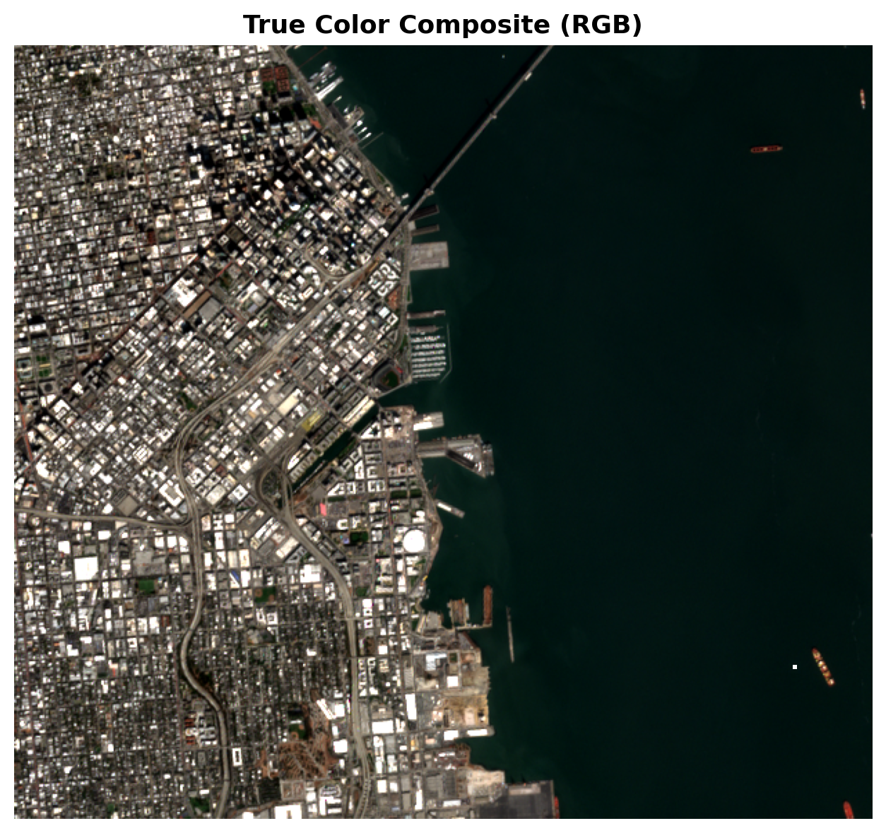
Figure 1: True Color RGB Composite from real Sentinel-2 data (San Francisco, Sept 2023). This is how the visible bands (B04, B03, B02) render before computing any indices.

Spectral Indices 101: Simple Math, Powerful Results

A spectral index is nothing fancy. It’s a mathematical combination of two or more bands designed to isolate a specific material property or landscape feature.

The formula is simple. The results are powerful.

Let’s walk through five indices you’ll use repeatedly in geospatial work.

NDVI: Normalized Difference Vegetation Index

Formula: (NIR − Red) / (NIR + Red)

Range: -1 to +1

• +1: Dense vegetation (tropical rainforest)
• 0.5–0.8: Healthy crops, forests
• 0.2–0.4: Sparse vegetation, shrubland
• 0: Bare soil
• < 0: Water, snow, built structures

Plants absorb red light (photosynthesis) and reflect NIR (cooling). Healthy plants = large NIR — Red difference.

Real-World Use Cases:

• Crop health monitoring: Farmers use NDVI time series to detect drought stress weeks before visible damage
• Forest mapping: Deforestation detection by tracking NDVI decline
• Urban sprawl tracking: Watch NDVI drop as vegetation disappears
• Disaster response: Post-flood assessment by mapping vegetation damage

import numpy as np
import rasterio

with rasterio.open('sentinel2_image.tif') as src:
    red = src.read(4).astype(float)    # Band 4 (red)
    nir = src.read(8).astype(float)    # Band 8 (NIR)

    # Compute NDVI with epsilon to avoid division by zero
    ndvi = (nir - red) / (nir + red + 1e-8)

    # Classify
    vegetation_mask = ndvi > 0.4

    print(f"Mean NDVI: {ndvi.mean():.3f}")

NDBI: Normalized Difference Built-up Index

Formula: (SWIR − NIR) / (SWIR + NIR)

Range: -1 to +1

• > 0.3: Urban/built-up (concrete, asphalt) - 0.0–0.3: Mixed urban/vegetation
• < 0: Vegetation, water

Buildings are made of concrete/asphalt with high shortwave-infrared reflectance. Vegetation has high NIR but low SWIR.

Use Cases:

• Urban mapping and change detection
• Construction site monitoring
• Infrastructure expansion tracking
• Slum detection (rapid informal settlement identification)

# NDBI highlights urban areas
swir = src.read(11).astype(float)  # Band 11 (SWIR)
nir = src.read(8).astype(float)
ndbi = (swir - nir) / (swir + nir + 1e-8)

urban_mask = ndbi > 0.3

NDWI: Normalized Difference Water Index

Formula: (Green − NIR) / (Green + NIR)

Range: -1 to +1

• > 0.3: Open water, wetlands
• 0.0–0.3: Mixed water/vegetation
• < 0: Dry land, urban

Water absorbs NIR and reflects green lights.

Use Cases:

• Water body mapping
• Wetland detection
• Flood mapping (post-disaster)
• Inundation extent assessment

# NDWI for water detection
green = src.read(3).astype(float)   # Band 3 (green)
nir = src.read(8).astype(float)
ndwi = (green - nir) / (green + nir + 1e-8)

water_mask = ndwi > 0.3

Other Indices Worth Knowing

• NDMI (Moisture Index): (NIR — SWIR) / (NIR + SWIR) → Crop stress, drought
• BSI (Bare Soil Index): (SWIR + Red — NIR — Blue) / (SWIR + Red + NIR + Blue) → Soil exposure, erosion
• GNDVI (Green NDVI): (NIR — Green) / (NIR + Green) → Fine-grained vegetation (better for crops)

Figure 2: Four spectral indices computed from the same Sentinel-2 scene. Each index isolates a different land cover property — vegetation, urban density, water bodies, and moisture content.

When Spectral Indices Beat Deep Learning: Know When to Stop Training and Start Computing

The biggest mistake in geospatial ML: reaching for deep learning before trying spectral indices (especially foundation models)

Here are four scenarios where indices outperform (or eliminate the need for) neural networks:

Scenario 1: You Have No Labeled Data

• Spectral indices: Unsupervised. No labels needed. Works out of the box.
• Deep learning: Requires 1,000–10,000 labeled examples.
• If you don’t have labels, indices are free. Fine-tuning a foundation model is better than training from scratch, but indices don’t require even that.

Scenario 2: You Need Real-Time or Edge Inference

• NDVI: One subtraction, one division, per pixel. Milliseconds on CPU.
• YOLOv8: 100M parameters, 50ms latency, GPU-only.
• If you’re analyzing satellite imagery on IoT devices or in edge scenarios, indices are the only option.

Scenario 4: You Need Explainability

• Deep learning: “Why did the model flag this area as urban?” Hard to explain. Regulators hate it.
• Indices: “NDBI > 0.3 = high built-up density.” Obvious. Stakeholder-friendly. Regulatory-compliant.
• If you’re building systems for governments, insurers, or compliance-heavy industries, interpretability matters.

When Deep Learning Is Worth ItThis code is production-ready.

Indices can’t do everything. They fail when:

• You need fine-grained classification (specific building types, damage assessment, crop varieties)
• You need pixel-level precision (exact building footprints, field boundaries)
• You have abundant labels (10K+ annotated examples) and want to extract value from them

Example: Detecting whether a building is “light damage,” “moderate damage,” or “destroyed” requires nuance that a simple spectral index can’t capture.

Combining Indices + Deep Learning: The Best of Both Worlds

You don’t have to choose between indices and deep learning. Here are three ways to combine them:

Indices as Preprocessing: Compute NDVI, NDBI, NDWI, stack them as features. Feed to a lightweight model (XGBoost, small CNN, ViT).

Result: Often outperforms raw bands alone, because you’ve given the model hand-crafted, physics-informed features.

Indices as Loss Signals: Train a segmentation model, but constrain the loss: Loss = standard_loss + λ * “preserve NDVI gradient consistency”

This keeps physics-based constraints in learned features. Models learn to respect spectral physics.

Indices for Post-Processing: Run model inference, then filter:

• “Remove all detections where NDVI < 0.2” (likely water/concrete, not vegetation)
• “Flag areas where NDBI > 0.4 as high-confidence urban”

This cleans up spurious predictions without retraining.

Hands-On Project: Build a Quick Change Detector

Detect Forest Loss in 20 Lines of Code

Let’s build something real. We’ll load two Sentinel-2 images (Year 1, Year 2), compute NDVI for each, and flag areas where NDVI dropped >0.3 (likely deforestation).

You’re monitoring a forest reserve. You want to detect illegal logging automatically. Data: Free Sentinel-2 images from USGS Earth Explorer or Copernicus Hub.

import numpy as np
import rasterio
import matplotlib.pyplot as plt

def compute_ndvi(red, nir):
    """Compute NDVI from red and NIR bands."""
    return (nir - red) / (nir + red + 1e-8)

# Load first date (2021)
with rasterio.open('sentinel2_2021.tif') as src:
    red_2021 = src.read(4).astype(float)
    nir_2021 = src.read(8).astype(float)
    ndvi_2021 = compute_ndvi(red_2021, nir_2021)

# Load second date (2024)
with rasterio.open('sentinel2_2024.tif') as src:
    red_2024 = src.read(4).astype(float)
    nir_2024 = src.read(8).astype(float)
    ndvi_2024 = compute_ndvi(red_2024, nir_2024)

# Compute change
ndvi_diff = ndvi_2024 - ndvi_2021
degradation_mask = ndvi_diff < -0.3  # Significant loss

# Statistics
degraded_pct = (degradation_mask.sum() / degradation_mask.size) * 100
print(f"Forest loss detected: {degraded_pct:.1f}% of area")

# Visualize
fig, axes = plt.subplots(1, 3, figsize=(15, 5))

# NDVI 2021
axes[0].imshow(ndvi_2021, cmap='RdYlGn', vmin=-1, vmax=1)
axes[0].set_title('NDVI 2021')
axes[0].colorbar()

# NDVI 2024
axes[1].imshow(ndvi_2024, cmap='RdYlGn', vmin=-1, vmax=1)
axes[1].set_title('NDVI 2024')
axes[1].colorbar()

# Degradation (red = loss)
axes[2].imshow(degradation_mask, cmap='Reds')
axes[2].set_title(f'Forest Loss (ΔNDVI < -0.3)')
axes[2].colorbar()

plt.tight_layout()
plt.savefig('forest_loss_detection.png')
print("Map saved to forest_loss_detection.png")

Figure 4: Change detection on real imagery. Left: NDVI in 2023. Center: NDVI in 2024. Right: areas where NDVI dropped >0.3 (potential vegetation loss). All from real Sentinel-2 data

Red areas = probable forest loss. Green areas = stable or recovering vegetation.

It works on real Sentinel-2 data. It’s fast (seconds, not hours). It’s interpretable (stakeholders understand what >0.3 ΔNDVI means).

That’s the power of spectral indices.