Why Traits Aren’t Easy to Predict and How We Can Predict Them: An Insight into Polygenic…
Table of Contents
Why Traits Aren’t Easy to Predict and How We Can Predict Them: An Insight into Polygenic Architecture, Statistical Limits, and Biological Complexity

Credit: Sangharsh Lohakare
Table of Contents
1: Abstract
2: Introduction
3: Polygenic Architecture: The Scale of the Problem
- 3.1 Many SNPs, Tiny Effects
- 3.2 The Infinitesimal Model
- 3.3 Missing Heritability
4: Statistical Barriers to Prediction
- 4.1 Linkage Disequilibrium
- 4.2 Sampling Noise
- 4.3 Overfitting and Shrinkage
- 4.4 Summary Statistics vs Individual-Level Data
5: Biological Complexity Beyond SNP Effects
- 5.1 Gene to Gene Interactions (Epistasis)
- 5.2 Regulatory Architecture
- 5.3 Environmental Effects
6: Prediction vs Causal Understanding
7: Functional Interpretation Challenges
8: Current Improvements and Future Directions
9: Conclusion
About Me
References
1: Abstract
While media such as GATTACA suggests that traits can be directly predicted from DNA, this is far from reality. Although the genotype (the genetic composition of an organism) is able to be read, interpreting it is much more difficult. It can be compared to reading a book in a language that is not fully understandable. Most phenotypes (the traits expressed in an organism) are multifactorial, meaning they are influenced by both genetic and environmental factors, making prediction difficult. To study the relationship between genotype and phenotype, Genome-Wide Association Studies (GWAS) are used, which analyze Single Nucleotide Polymorphisms (SNPs), or single-base changes in DNA. These studies identify statistical associations between genetic variants and traits, rather than direct cause-and-effect relationships. Researchers also use Linkage Disequilibrium (LD) to measure how often certain genetic variants are inherited together. However, LD reflects correlation between SNPs and alleles (variations of a gene), not necessarily which variant is biologically responsible for a trait. Early predictive models assumed that all genetic variants contributed equally to a phenotype, but newer models recognize that some regions of the genome have larger effects than others. While these improvements have increased accuracy, prediction remains limited. Models that perform well on known datasets often fail to generalize to new individuals, with accuracy heavily influenced by factors such as ancestry and sample composition. Although ongoing improvements — such as larger datasets, better statistical models, and multi-trait analysis — continue to advance the field, the complexity of genetic architecture and environmental influence makes precise phenotype prediction a significant challenge.
2: Introduction
The primary challenge in modern genomics is not our ability to edit DNA, but our inability to predict the resulting phenotypes. Scientists have reached a paradox in biotechnology: tools like CRISPR-Cas9 allow us to rewrite the genetic code with extreme precision, yet our capacity to forecast the effects of those edits has stalled. This gap in prediction is most evident in polygenic traits, where researchers can identify statistical associations through GWAS but struggle to establish direct biological causality. A GWAS is a systemic genomic scan of an organism’s DNA, specifically identifying SNPs that correlate with specific traits (Ma & Zhou, 2021). While these studies have successfully connected genomic regions to phenotypes, they often fail to explain exactly how it contributes to the phenotype. GWAS leverages Linkage Disequilibrium (LD), which is the non-random association of alleles at different loci. In simpler terms, LD means that certain genetic variants are inherited together more often than expected by chance, allowing researchers to use ‘tag SNPs’ to represent entire blocks of the genome. To improve these predictions, researchers rely on LD to identify which SNPs are inherited together. By leveraging LD, scientists can build models to estimate phenotypic outcomes more accurately. Despite these advancements, the “instruction manual” for complex human biology remains difficult to read.

Manhattan plot visualizing genomic expression. The red line represents the threshold of statistical significance for a specific trait. Credit: Bernal Rubio et al.
3: Polygenic Architecture: The Scale of the Problem
3.1 Many SNPs, Tiny Effects
Most complex traits such as height, eye colour, and lifespan are not decided by one gene, it is usually the result of polygenic architecture. Polygenic architecture is essentially the biological blueprint that explains how traits are influenced by several genetic variants. The genotype of these genes vary from person to person. In other words, there are a multitude of SNPs within a genome for each person which have a multitude of negligible effect sizes contributing to the final trait. SNPs contribute small phenotypic variance because they only change one nucleobase from the entire genome, but since there are multiple SNPs within multiple people, it becomes much more difficult to associate genes and traits. In other words, each SNP has an infinitesimal (very small) effect on the final outcome. This limits prediction simply because there are too many SNPs to keep track of. It becomes difficult to organize and connect the SNPs to a trait, especially if they’re not in LD with other SNPs, as it requires aggregating massive amounts of data points, increasing statistical noise.
3.2 The Infinitesimal Model
To combat the difficulty of connecting SNPs to traits, researchers developed a model that is used to explain how complex traits are inherited, known as the infinitesimal model. The model states that a trait is influenced by thousands of tiny genetic variations, each having an infinitesimal effect. When scientists use mathematical tools to predict traits, they often use what they call a “pseudo-infinitesimal” model. In this math model, they assume every single variation in the genome has some effect on the trait and that all the effects are roughly the same magnitude. An example of this is if someone has 1 million variations, the model might assume each one only explains one-millionth of the trait (Gouddard et al., 2016).
3.3 Missing Heritability
For a long time, researchers were confused because they could only find a few genes for traits like height, which only explained about 5% of the variation (Gouddard et al., 2016). For a trait like human height, twin studies suggest a heritability of ~80%, yet early GWAS results only accounted for ~10 to 20% (Meuwissen & Goddard, 2010). This discrepancy is known as ‘Missing Heritability,’ caused by rare variants, structural variations, and epistasis that common SNP arrays fail to capture.. This was called the missing heritability problem. Missing heritability is the lack of connection between high trait estimates from family studies and the much lower estimates from GWAS. It suggests identified common DNA variants do not fully explain inherited phenotypic variance. The potential causes for missing heritability includes total vs SNP heritability, rare variants, gene to gene interactions (epistasis), and non-coding and/or epigenetic factors — anything influencing the amount of expression of genes. Total heritability is the proportion of the overall variation in a trait that is caused by all genetic factors and it is generally estimated by looking at families or twins. However, SNP heritability is a narrower measure that refers specifically to the proportion of variation that can be explained by common Single Nucleotide Polymorphisms (SNPs).
How the number of SNPs included help explains phenotypic variation. Credit: Makowsky et al.
This matters because of how much each type explains: height has a total heritability of ~80%, yet initial studies found that common SNPs only explained about 45% of the variance. This gap (A.K.A. missing heritability) exists because common SNPs don’t capture every type of genetic variation, and many individual genetic effects are too small to be detected by most mathematical models. Rare variants are genetic differences that occur very infrequently in the population, often defined as being present in less than 0.1% or 1% of people. Unlike common variations, which usually have tiny effects, rare variants can be “highly penetrant,” meaning a single rare variant can have a very large impact on an individual’s risk for a disease. Scientists believe rare variants are a major reason for “missing heritability” because standard SNP tests often miss them. While they don’t affect many people across the whole population, discovering them is highly valuable for the specific individuals who carry them, as they provide a much clearer “meaning” for that person’s health. With structural variants, they involve large-scale changes to the DNA sequence, rather than just a single nucleobase change. Like rare variants, structural variants are considered a primary suspect in the “missing heritability” mystery because they are often undetected by standard tools designed to look for SNPs. Scientists try to combat this with mathematical tools to create more accurate and complete prediction models. Despite all this, even perfect measurement of common SNPs explains limited variance (Campos et al., 2018).
4: Statistical Barriers to Prediction
4.1 Linkage Disequilibrium
Linkage disequilibrium indicates that specific alleles are correlated, often because they are physically close on the same chromosome, restricting rearrangement of genes for different alleles. When scientists run a study and see that a specific SNP is linked to a trait, they don’t immediately know if that SNP is the cause or if it’s just in an inherited “block” and in LD with a group of other SNPs. The actual cause SNP is known as the causal variant and they are the actual mutations that change how a protein is made or how a gene is turned on or off, directly affecting a trait or disease risk. The SNPs that don’t change anything within the proteins are called tagging SNPs and they are more like bookmarks/proxies to nearby causal variants. Often, they are able to “tag” a causal variant because they are correlated with a causal variant in a similar location. Standard genetic tests usually use a set of common “tagging” SNPs to scan the genome. They can tell that a “culprit” is in a certain genetic neighborhood, but they don’t always point to the exact house. However, it’s not as simple as using the tagging variant to find the causal variant. There are several reasons causal SNPs can’t be found easily. An example of this is there being too many suspects for causal variants. If five SNPs are always inherited together, they are statistically indistinguishable. A computer model can tell the causal variant is one of those five, but it has no mathematical way to pick the single biological cause without further experiments. Another reason is that there are too many causal SNPs. For most complex traits, there isn’t one “big” causal SNP. Instead, there are thousands of tiny ones. Many of these individual variants explain less than 1% of the trait. It is very hard to distinguish such a miniscule biological target from random, unrelated statistical data or sampling error. Furthermore, the SNP can be in a locus that is not common within the genome. Scientists used to look mainly at the parts of DNA that code for proteins. However, research shows that the majority of causal mutations for complex traits actually live in regulatory regions, which control how much certain genes are expressed. Researchers are still learning how to comprehend how these regulatory regions work, which makes identifying the causal SNPs much harder.
4.2 Sampling Noise
Sampling noise is like the “static” on a radio. Because scientists usually study a small group of people rather than every person on Earth, the results can be slightly different every time just by chance. If a study is too small, it is very hard to tell if a genetic variation is actually important or if it just looks important because of random luck. To filter the noise, researchers need massive sample sizes. A way to measure unrelated data, is by something called standard errors. This is a measure of how much “noise” is in a specific measurement. A smaller standard error (often shown as a narrow confidence interval) means the scientists have a more precise and trustworthy estimate of a gene’s effect.

Standard error measurement from training models. Credit: Pasanuic & Price
Other measurements that are used are Z-scores and P-values. Z-scores are the number of deviations above or below an average value. Z-scores are used to compare different genetic variations. P-values tell the probability that a result happened purely by chance. Because geneticists test millions of DNA variations at once, they have to use extremely strict P-values (usually less than 0.00000005 or 5 × 10^-8) to make sure they aren’t being fooled by random patterns. Sampling noise can also occur with something known “winner’s curse.” Winner’s curse happens when scientists usually only report the SNPs that had the most impressive, significant results in their study. Because of random sampling noise, the “winners” in a specific study often have their effect sizes overestimated. They look much more powerful than they actually are because their “natural” effect was randomly boosted in that specific group of people. To beat the Winner’s Curse, scientists must test those same “winning” SNPs in a completely independent dataset to see if the effect is still as strong when the “luck” is removed.
4.3 Overfitting & Shrinkage
Moving into the more advanced mathematical side of genetics, it helps to think of models as “filters” that try to separate the real genetic signals from the random noise. In most genetic studies, scientists face a massive math problem: they have millions of SNPs (p) but only a few thousand people (n). Because there are way more “instructions” than there are people to study, a standard computer model will try to be “too perfect.” This can lead to overfitting, which is when a model “memorizes” the specific people and noise in the original study, rather than learning the general rules of biology. An overfitted model looks 95% accurate on the people it already knows, but it fails miserably (dropping to 15% to 35% accuracy) when trying to predict a new person. In an attempt to move away from overfitting, shrinkage is utilized to regulate the “noise” that comes from statistical data. Shrinkage is when a math model is told to “pull” the estimated effect of every SNP toward zero, in other words shrinking its value. The logic is if a SNP has a very tiny, weak link to a trait, the model assumes it’s just noise and “shrinks” its effect to zero. Only the SNPs with signals strong enough to “resist” this pull are kept as part of the prediction. A commonly used model today is the Genomic Best Linear Unbiased Prediction (GBLUP). It works by using a “Genomic Relationship Matrix” to see how similar two people are based on their entire DNA. However, this model’s flaw is that it assumes every SNP has an effect and that all these effects are pseudo-infinitesimal. Because it treats every part of the DNA as equally important, it can’t properly account for the specific regions that might be way more important than others. In contrast, smarter models called Bayesian models are being utilized for predictions. They are often more accurate because they don’t assume every SNP is equal. They work by starting with a “prior,” which is a set of biological assumptions. The main difference is instead of assuming every SNP does something, a Bayesian model like BayesR might assume that 95% of DNA does absolutely nothing for a specific trait, while the other 5% has varying levels of impact. By putting a weight on some genes, these models are much better at mapping where the real biological action is happening. Despite the advancement in models, it still doesn’t mean prediction equals to causal identification. This means that knowing that something will happen is not the same as knowing why it happens. A predictive model only needs to find correlation patterns. For example, a tagging SNP might be 100% accurate at predicting a disease, even if that specific SNP is biologically useless. It works simply because it is in LD with the real causal mutation. A model can be built that is great at predicting who might get Type 2 Diabetes without actually understanding the mutation that causes it. To find the causal variant, scientists have to go beyond math and do functional studies to see which mutation actually changes a protein or influences a gene’s expression.
4.4 Summary Statistics vs Individual-Level Data
Summary statistics are the average statistics done from studies whereas the individual-level data is specific to one person only. To understand the difference between summary statistics and individual-level data, imagine the difference between a high school’s final report card for the whole class versus having every student’s actual exam papers. Individual-level data includes the specific genotype and trait values for every single person in a study. It is very high-standards for research because it allows for the most detailed math, but it is often hard to get because of privacy concerns and the massive computer power needed to process it. Summary statistics however are simplified “per-allele” results. Instead of seeing every person, scientists just see the average effect of each SNP and the standard error. These are much easier to share and cheaper to analyze because the math model difficulty doesn’t increase as add more people are added to the study. While summary statistics are great for sharing, they have specific limits. Unlike individual data, summary statistics cannot capture “non-linear” relationships between SNPs. They see the SNPs one by one rather than seeing the complex “blocks” of DNA (haplotypes) that individuals actually carry.

The graph shows an ideal diagnostic scenario compared to the pattern expected using random predictions. Credit: Schrodi et al.
Additionally, For certain tasks, like studying very rare variants, summary statistics aren’t enough. Scientists often need the actual “in-sample” data (the original genotypes) to avoid getting false-positive results. Because summary statistics don’t tell how different SNPs are linked together, scientists have to “guess” that linkage using an LD Reference Panel. The way it works is with scientists using a separate group of people as a template for what typical human DNA linkage looks like. With this approach, the risk is if the people in the template study have a different ancestry than the people in current study, the estimates will be wrong. Because these reference templates are usually small (usually only a few hundred or thousand people), scientists have to use a trick called regularization. Regularization involves cleaning up the math, such as by assuming SNPs very far apart have zero connection to each other, to make the results more reliable. In continuation, one of the biggest problems with using summary statistics for advanced predictions is noise accumulation. There is always a tiny difference between the DNA linkage in a reference panel and the real linkage in the current study group. As one tries to calculate the effects of millions of SNPs across the entire genome, these tiny errors start to add up, eventually making the final prediction totally inaccurate. To stop this noise from building up, newer tools (like MegaPRS) use a “sliding window” approach. Instead of looking at the whole genome at once, the computer only looks at a tiny chunk (about 3 million base pairs) at a time, makes the calculation, and then moves to the next chunk. This prevents the errors from one part of the genome from ruining the math for the rest of the DNA.
5: Biological Complexity Beyond SNP Effects
5.1 Gene to Gene Interactions (Epistasis)
Understanding epistasis can be done with an analogy of DNA as team workers. In a simple model, each worker does their job independently, and the individual work is simply added to get the final result. Epistasis is when the workers have to interact or use teamwork to get the job done. One worker might be useless unless another specific worker is also present to help them. Epistasis is a common non-additive effect. In genetics, additive means that every DNA variation has a fixed “value” that it adds to a trait, no matter what other genes someone has. Non-additive effects, however, happen when that value changes depending on the genetic background. Epistasis being a non-additive effect means the effect of one gene is hidden or modified by another gene (Schrodi et al., 2014). Another example of a non-additive effect is dominance, which is when 2 versions of a gene inherited from both parents interact with each other at the same location. The reason most linear models struggle is because of these non-additive effects. Most of the common mathematical tools used today, such as GBLUP or standard regression, are linear models. These models are designed to find the “average” effect of each gene across a whole population. They struggle with epistasis because of several reasons such as the assumption of independence, the “search space” problem, need for massive data, and missing heritability. Starting with the assumption of independence, linear models assume that each SNP works alone. They can be thought as a calculator that only has a plus button, they are great at adding up thousands of tiny independent effects, but they cannot easily calculate “if A and B are both present, then multiply the result.” Moving on to the “search space” problem, there are millions of SNPs in the human genome. While it’s easy for a computer to check them one by one, it is computationally inefficient to check every possible pair or triplet of SNPs to see if they interact. This is why mathematical models involve matrices and vectors: because they handle a massive amount of SNPs and data that matrices and vectors are necessary to organize them. The number of combinations is simply too massive for standard computers to handle easily. Furthermore to the need for massive data, to prove the epistasis occurance isn’t a fluke, scientists need much larger sample sizes than they do to find simple additive genes. Without enough people in a study, the signal of an interaction gets lost in statistical noise. Finally to missing heritability, because linear models don’t consider complex interactions, they often fail to explain the full genetic cause of a trait. This is a major reason why scientists believe some heritability remains missing — it is because it is hidden in interactions that current math can’t see. To attempt to move away from these flaws, researchers are trying to develop new tools. Some use machine learning (like Random Forests or Neural Networks) to find patterns that a simple linear model would miss. Others use tools like MultiBLUP, which can be told to look for specific categories of genes or pathways where interactions are biologically likely to happen.
5.2 Regulatory Architecture
The regulatory architecture of the genome refers to the system that controls that influence when, where, and how much of a protein a gene produces. Research shows that the majority of mutations affecting complex traits are located in these regulatory elements rather than in the genes themselves. Several concepts can be used to study regulatory architecture, for example eQTLs. An expression Quantitative Trait Locus (eQTL) is a specific genetic variation that is associated with the expression level of a gene. Most eQTLs studied are cis-acting, meaning they are located very close to the gene they regulate and affect the expression of the gene on that same chromosome. Scientists use Transcriptome-Wide Association Studies (TWAS) to integrate eQTL data with GWAS results (Kerimov et al., 2021).

Process of conducting a TWAS and eQTL analysis. Credit: Kerimov et al.
This allows them to predict whether a person’s genetic risk for a disease is actually being driven by changes in how their genes are being regulated. Using eQTLs can be more powerful than standard genetic tests because the gene expression is often much stronger and clearer than the final trait. The regulatory architecture is highly tissue-specific, meaning a genetic regulations might be active in the brain but completely silent in the liver. By overlapping genetic risk signals with maps of active regulatory regions, researchers can identify the critical cell types where a disease actually starts. An example of this is polygenic signals for platelet count are specifically enriched in regulatory regions active in the cell lineage that leads to platelets. This concept also applies to alleles where one version of a gene is more active than the other in a specific tissue. Studies show that about 89% of genes in some species exhibit this kind of specific imbalance in at least one tissue. Timing of when genes are active is vital to understanding the genetic architecture of traits. In human studies, accounting for developmental stages (like teenagers who are still growing) is necessary to avoid adding “noise” to genetic models, as the regulatory systems in a growing child differ from those in an adult. Using biobanks linked to medical records allows scientists to perform historical prospective studies. They can track how a person’s regulatory architecture correlates with the actual timing of a disease’s onset or how a trait changes over their lifetime. In evolution, traits under strong natural selection often involve regulatory changes that drive alleles to low frequencies in a population. This suggests that the timing and precision of gene regulation are essential for an organism’s survival and fitness.
5.3 Environmental Effects
To understand why DNA isn’t “destiny,” it helps to think of genetic code as the blueprints for a house, while the environment is the construction crew, the weather, and the neighborhood. No matter how perfect the blueprint is, the final house depends on who builds it and what happens to it over time. In other words, traits can be affected by more than DNA, it can also be affected by the environment through different interactions. Gene to environment interactions happen when a specific genetic variation only matters if in a specific environment, known as interaction co-conspirators. The context matters though; a gene can give a negative effect under one environment, but that same gene might have no effect (or even a positive one) in another environment. For example, some genetic risks for a major depressive disorder are only “activated” or made worse by specific stressful life events or childhood trauma. A similar concept is phenotypic plasticity. This is the idea that one genotype can produce different phenotypes based on the environment. For example, in height studies, researchers have to account for the fact that teenagers are still growing; this creates “noise” in the data because their current height isn’t their “final” genetic height yet. However, some factors classified as the “environment” might actually just be stochastic events, which are purely random biological accidents that DNA cannot predict. Examples of the environment that don’t relate to immediate surroundings are socioeconomic and lifestyle factors. These are external forces that act on biology regardless of the “blueprints.” Researchers use tools like the Townsend Deprivation Index to measure how wealth and neighborhood quality affect health outcomes (Zhang et al., 2021). A person might have healthy genes, but living in a high-pollution or high-stress area can devalue those genetic advantages. Additionally, Factors like smoking, diet, and exercise are massive external variables (Schrodi et al., 2014). For a trait like age-related macular degeneration (an eye disease), adding info about a person’s smoking habits to their genetic data makes the prediction much more accurate than using DNA alone (Wray et al., 2013).
The main difference between gene to environment and phenotypic plasticity is gene to environment happens when the effect of a specific genetic variation depends on the environment, meaning a genetic variant might be a high-risk factor in one environment but have zero effect in another. However, phenotypic plasticity means one genotype can produce more than one phenotype, which means the final result changes even if the genotype stays exactly the same. It includes purely random biological accidents that DNA simply cannot predict. An analogy that can be used to demonstrate gene to environment interaction is a seed that can only grow if it’s planted in a specific soil, but for phenotypic plasticity, that plant grows crooked, regardless of species. This means that gene to environment interactions are hard to predict as both the DNA and specific environment need to be known, whereas phenotypic plasticity is impossible to predict because one can’t predict the stochastic events (Bernal Rubio et al., 2015).
In short, a genetic predictor is a probabilistic tool, not a crystal ball. It can tell one the baseline risk, but it cannot see the infections that can be caught, the food one will eat, or the random accidents that will shape someone’s health.
6: Prediction vs Causal Understanding
The goal of a predictive model is statistical accuracy, but this does not always lead to biological understanding. In many cases, it’s possible to predict a phenotype successfully without ever identifying the causal variants responsible for it. This happens because models prioritize statistical optimization — they look for any signal, even if that signal comes from a tagging SNP that is simply located near the actual mutation. For a researcher focused on prediction, a high correlation is a success. However, for a researcher focused on gene editing, a model that predicts well but lacks causal discovery is functionally useless, as editing a non-causal SNP will not result in a phenotypic change. Models are able to be accurate without knowing biological cause because of SNPs in LD. If a tagging SNP is in LD with a causal SNP, it is often sufficient to predict who is at risk for a disease since a model only needs to find a general correlation. It does not need to know which chemical pathway is broken or which protein is shaped incorrectly to give a useful risk score. While it is easy for a computer to see that, for example, an SNP is linked to height it is very difficult for scientists to prove that the same SNP influences height. If five SNPs are always inherited together in a tight block, they are statistically indistinguishable, meaning it’s not possible to find the SNP that is the biological cause for the trait. The math model might pick one of them as a great predictor, but that doesn’t mean it’s the biological cause, it might just be pure chance that it’s in LD with the cause SNP (Gouddard et al., 2016). To optimize with the intent to find causal SNPs, scientists can look for eQTLs by doing a TWAS. By aggregating GWAS data, researchers develop Polygenic Risk Scores (PRS). These models act as a statistical summary of an individual’s genetic liability. However, a high PRS can predict a trait without identifying its biological etiology. By doing this, researchers can test whether a person’s risk for a disease is actually driven by a specific gene. If a DNA variant matches the pattern of a gene’s expression and the final disease trait, it is a very strong candidate for a biological cause. However, a high PRS can predict a trait without identifying its biological causes. For gene editing technologies like CRISPR-Cas9, this is a critical bottleneck since a model may predict who is at risk for a disease, but it cannot tell the editor exactly which base pair must be modified to fix it (Pasaniuc & Price, 2016).

Flowchart of SNP-based analysis. At each stage data is needed in, a process is applied and a result is generated. Credit: Wray et al.
Additionally, because different ethnic groups have different SNPs in LD with each other, a tagging SNP that works in South Asians might not work in East Asians. However, the true biological cause should be consistent across all humans. By comparing data from multiple ancestries, scientists can find the average of the total signals from random tagging SNPs and pinpoint the one variant that remains linked to the trait across all groups. A biological cause is often pleiotropic, meaning it affects more than one trait. For example, a variant that changes how a specific phosphorus-transporting protein works might affect both milk volume and the chemical concentration of that milk (Gouddard et al., 2016). When scientists see a single SNP having a strong impact on multiple biologically related traits, they gain much higher confidence that they have found a true causal mechanism.

How differenet models’ prediction accuracy respond change when summary statistics are used. Credit: Zhang et al.
For the intention of optimizing prediction, Bayesian models such as LDAK-Bolt-Predict or the BayesR are severely beneficial for this goal (Zhang et al., 2021). Additionally, optimization with consideration of gene to environment interactions, phenotypic plasticity, epistasis, or epigenetics can enhance phenotype prediction accuracy. This distinction is vital for the future of therapeutics. While a predictive model might tell us who is at risk, only causal discovery tells a researcher which exact nucleotide to target with CRISPR-Cas9 to reverse a disease phenotype.
7: Functional Interpretation Challenges
Attempting to understand the function of certain SNPs or how it translates into its final trait is one of the greatest challenges of modern genetics. While studies have identified tens of thousands of associated variants, actually proving why they affect health is difficult for several reasons. Most genetic variations linked to diseases do not actually change the amino acids of proteins. In fact, approximately 39% of disease-associated variants are intergenic (found between genes) and 36% are intronic (found inside non-coding parts of genes) (Schrodi et al., 2014), where the rest are found within the amino acids of proteins. Because these variants don’t change a protein’s structure, they often have no obvious biological function, making them much harder to study than mutations that directly break a gene. Additionally, Finding the exact “culprit” mutation is difficult because of LD. When a study finds a strong signal, there are often dozens of nearby SNPs that are also associated with the trait simply because they are essentially “physically stuck” to the real causal variant. If several variants are in high LD, mathematical models often cannot determine which one is the true cause and which are tagging SNPs. Even with large datasets, the variant with the highest statistical score may not be the actual causative mutation due to random sampling noise.
To continue, making sense of thousands of tiny genetic effects requires scientists to use something known as pathway enrichment to see if associated SNPs fit within specific biological classifications or pathways. Pathway enrichment is a process that identifies biological pathways or functions, such as metabolic pathways or gene ontology terms — standardized vocabulary to describe gene product functions — that are overrepresented in a set of genes (Bass et al., 2013). By fusing SNP data with known biological pathways, researchers can identify which systems (like the immune system or metabolism) are likely being disrupted. However, for many traits, variants are clustered across hundreds of different loci and pathways, making it hard to pinpoint to a single dysfunctional process. Scientists use colocalization — a statistical method used to determine if two or more traits share the same causal genetic variant at a specific genomic location — to see if a genetic signal for a disease overlaps perfectly with a signal for gene expression (which leads to the actual protein being made). The “instructions” for DNA is incredibly complex because regulatory elements. Evidence suggests that the majority of mutations affecting complex traits live in these regulatory switches rather than in the genes themselves (Gouddard et al., 2016). A genetic switch might be broken in the brain but work perfectly in the heart, meaning scientists have to test the DNA in many different cell types to find the mechanism (Gouddard et al., 2016).
Furthermore, allele-specific expression can occur, which is when one inherits more than one version of a regulatory element, but one is more active than the other. Research shows that 89% of genes show this kind of specific imbalance in at least one tissue, adding a massive layer of complexity to finding the true biological cause (Makowsky et al., 2011).
8: Current Improvements & Future Directions
To summarize the steps scientists can take, it’s important to consider that most of the solutions apply with specific goals in mind, for example there can be a goal either have the goal to improve their prediction of complex traits or finding causal genetic variations, but some of these can apply with both cases as well. To begin, scientists can try to get as large of a sample size as possible, especially from family members. By doing this, it is possible to not only understand the true effect of a genetic variation’s effect, but also filter out any irrelevent noise and be able to focus more on the biological signals from the causal SNP. This helps in both cases since it ensures the results from are more accurate, meaning it will help predict by looking for the causal SNP through the tagging SNPs, and it will help look for the cause by creating more precise results from looking for eQTLs through a TWAS. In continuation, multi-omics integration is way to find biological causes. Multi-omics integration is the process of combining different layers of biological information to get a complete picture of how a disease or trait works. While a standard genetic study looks only at DNA coding, multi-omics adds other layers. For example, with transcriptomics scientists study eQTLs to see how much DNA variations affect how much of its protein product a gene makes. Additionally, with epigenomics, chemical markers on DNA like histone marks are used to regulate gene expression. Furthermore, proteomics and metabolomics are used to measure current level of proteins and metabolites in blood. These are called “dynamic markers” because, unlike static DNA, they reflect current status of DNA in one’s body. Multi-omics integration is necessary to consider because most disease-linked DNA variations are non-coding, making their function more ambiguous. By utilizing both these layers together, researchers can identify the specific biological pathways that are mutated. Moving on, fine mapping is also a major factor to enhance. Fine-mapping is the statistical process of pinpointing the exact causal variant from a group of nearby candidates in LD (Pasaniuc & Price, 2016). Fine-mapping aims to move from simple correlation (knowing a neighbor is linked) to causal identification (proving which DNA letter is the cause) to enable further laboratory experiments. Additionally, machine learning can be utilized to find patterns that are difficult to spot. As stated before, standard models assume each gene works independently. However, biology is often about teamwork (shown through epistasis), where one gene only matters if another gene is also present. Scientists are using ML tools like Random Forests, Neural Networks, and Support Vector Machines to detect these complex interactions (Bass et al., 2013). These tools can look at thousands of genetic variations in parallel to see how they interact, which is computationally too hard for traditional math. Moving forward, current medicine often groups diseases by their visible symptoms like stomach pain, but that pain could easily be caused by five different biological mutations. Machine learning aids by looking at the molecular makeup of the DNA to determine classification, instead of using just their symptoms. This approach allows for precision medicine, where a doctor can treat the exact biological cause of a disease rather than just the symptoms. Furthermore, despite large samples being optimal, it can be a strain computationally. Advanced algorithmic techniques like Variational Bayes and Coordinate Descent are being integrated into new tools (like MegaPRS and LDAK) (Speed & Balding, 2014). These ML-inspired methods allow scientists to build highly accurate prediction models in a few hours on a standard desktop computer, whereas older methods might have taken weeks or required a supercomputer. Finally, a major challenge in current genetic research is that some models built using one population (often individuals of European descent) typically perform poorly when applied to other groups, such as individuals of African, East Asian, or South Asian ancestry. This is because LD varies significantly across different ethnic groups. A SNP that is a great “proxy” or “tag” for a disease in Europeans might not be linked to that disease in another group (Meuwissen & Goddard, 2010). This is the reason sample sizes must increase so that more versatile models are developed that are applicable to all ancestries. While population diversity makes prediction harder, it is actually a powerful tool for fine-mapping. Because different populations have different DNA groups, scientists can compare them to see which genetic variation remains linked to a trait across all groups. The true biological cause should be consistent across all humans, while the random tagging SNPs will vary.
Posterior probability results from BayesR model. Credit: Goddard et al.
Models like the Bayes RC or MultiBLUP can help move away from models that assume everyone’s DNA works the same. This approach has been shown to significantly reduce the number of potential suspects in a genomic region, helping scientists pinpoint the real biological source (Bernal Rubio et al., 2015). Many modern genetic tools require LD Reference Panels to account for the gap of missing heritability, however if the template used doesn’t match the same ethnicity of the individual who’s DNA is being studied, it can be inaccurate and leads to false-positive results. Scientists need to create larger and more diverse reference templates to ensure that techniques like estimating missing DNA nucleotides work correctly for everyone. Finally, it is emphasized that a “one size fits all” approach to genetic medicine won’t work. Applying predictive models to diverse clinical populations is essential to understand their limitations and ensure they provide improved health outcomes for everyone, not just those from the groups that have been studied the most.
9: Conclusion
To summarize, phenotype prediction remains one of the most challenging aspects of modern genomics. The relationship between genotype and phenotype is not a simple linear map, but a vast, interconnected network of polygenic architecture. With millions of variations producing infinitesimal effects, the task of organizing these patterns would be impossible without the integration of Bayesian frameworks and machine learning. However, statistical success does not always equal biological understanding. The presence of LD continues to obscure true causal variants, leaving researchers with a sea of candidates that “ride along” actual causal variants and complicate functional discovery. Furthermore, it’s important to contend with “undetectable” part of biology: the environmental interactions, epistatic networks, and epigenetic regulations that introduce non-genetic variance. Moreover, the future of personalized medicine and CRISPR-Cas9 depends on what researchers can do now with new advancements. Scientists currently possess a “molecular scalpel” capable of rewriting the code of life, but they are still learning how to read the instructions. The full potential of gene editing will remain hindered by our inability to predict the consequences of a single edit unless the gap between statistical correlation and biological causality is birdged. The difficulty of phenotype prediction is not a failure of genetics, but rather, it is a profound reflection of the staggering complexity of life itself. Realizing that the genome is not a simple, static blueprint, but a dynamic network that simply has not been fully explored yet will significantly aid scientists comprehend the true nature of the relationship between the genotype and phenotype.
About Me
My name is Ankit Chandna, a 16 year-old researcher in gene editing and how control on it can be further enhanced. If this article was interesting to you, consider checking out my other articles!
References
Bass, A., Gondro, C., Werf, J. V., & Hayes, B. (2013). Genome-Wide Complex Trait Analysis (GCTA): Methods, Data Analyses, and Interpretations. Academia. Retrieved March 14, 2026, from https://www.academia.edu/11753226/Genome_Wide_Association
Bernal Rubio, Y. L., Gualdró, J. L., Bates, R. O., Ernst, C. W., Nonneman, D., Rohrer, G. A., King, A., Shackelford, S. D., Wheeler, T. L., Cantet, R. J. C., & Steibel, J. P. (2015, November 26). Meta-analysis of genome-wide association from genomic prediction models. Wiley Online Library. Retrieved March 19, 2026, from https://onlinelibrary.wiley.com/doi/full/10.1111/age.12378
Campos, G. D., Vazquez, A. I., Hsu, S., & Lello, L. (2018, August 20). Complex-Trait Prediction in the Era of Big Data. ScienceDirect. Retrieved March 23, 2026, from https://www.sciencedirect.com/science/article/abs/pii/S0168952518301252?fr=RR-2&ref=pdf_download&rr=9e40b2dd5a5339cc
Gouddard, M. E., Kemper, K. E., MacLeod, I. M., Chamberlain, A. J., & Hayes, B. J. (2016, July 1). Genetics of complex traits: prediction of phenotype, identification of causal polymorphisms and genetic architecture. The Royal Society Publishing. Retrieved March 21, 2026, from https://royalsocietypublishing.org/rspb/article/283/1835/20160569/84471/Genetics-of-complex-traits-prediction-of-phenotype
Kerimov Nurlan, Hayhurst James D., Peikova Kateryna, Manning Jonathan R., Walter Peter, Kolberg Liis, Samoviča Marija, Pandian Sakthivel Manoj, Kuzmin Ivan, Trevanion Stephen J., Burdett Tony, Jupp Simon, Parkinson Helon, Papatheodorou Irene, Yates Andrew D., Zerbino Daniel R., & Alasoo Kaur. (2021, September 6). A compendium of uniformly processed human gene expression and splicing quantitative trait loci. Nature Communications. Retrieved March 18, 2026, from https://www.nature.com/articles/s41588-021-00924-w
Ma, Y., & Zhou, X. (2021, November). Genetic prediction of complex traits with polygenic scores: a statistical review. ScienceDirect. Retrieved February 22, 2026, from https://www.sciencedirect.com/science/article/abs/pii/S0168952521001451?fr=RR-2&ref=pdf_download&rr=9e40ba5b3b0d39cc
Makowsky, R., Pajewski, N. M., Klimentidis, Y. C., Vazquez, A. I., Duarte, C. W., Allison, D. B., & Campos, G. D. (2011, April 28). Beyond Missing Heritability: Prediction of Complex Traits | PLOS Genetics. PLOS Genetics. Retrieved February 25, 2026, from https://journals.plos.org/plosgenetics/article?id=10.1371/journal.pgen.1002051
Meuwissen, T., & Goddard, M. (2010, March 15). Accurate Prediction of Genetic Values for Complex Traits by Whole-Genome Resequencing. National Library of Medicine. Retrieved March 12, 2026, from https://pmc.ncbi.nlm.nih.gov/articles/PMC2881142/pdf/GEN1852623.pdf
Pasaniuc, B., & Price, A. L. (2016, November 18). Dissecting the genetics of complex traits using summary association statistics. National Library of Medicine. Retrieved March 5, 2026, from https://pmc.ncbi.nlm.nih.gov/articles/PMC5449190/pdf/nihms858267.pdf
Schrodi, S. J., Mukherjee, S., Shan, Y., Tromp, G., Sninsky, J. J., Callear, A. P., Carter, T. C., Ye, Z., Haines, J. L., Brilliant, M. H., Crane, P. K., Smelser, D. T., Elston, R. C., & Weeks, D. E. (2014, June 1). Genetic-based prediction of disease traits: prediction is very difficult, especially about the future†. Frontiers. Retrieved March 17, 2026, from https://www.frontiersin.org/journals/genetics/articles/10.3389/fgene.2014.00162/full
Speed, D., & Balding, D. J. (2014, June 24). MultiBLUP: improved SNP-based prediction for complex traits. CSH Press Genome Research. Retrieved March 9, 2026, from https://genome.cshlp.org/content/24/9/1550.short
Wray, N. R., Yang, J., Hayes, B. J., Price, A. L., Goddard, M. E., & Visscher, P. M. (2013, July 15). Pitfalls of predicting complex traits from SNPs. National Library of Medicine. Retrieved March 12, 2026, from https://pmc.ncbi.nlm.nih.gov/articles/PMC4096801/pdf/nihms589441.pdf
Zhang, Q., Privé, F., Vilhálmsson, B., & Speed, D. (2021, July 7). Improved genetic prediction of complex traits from individual-level data or summary statistics. Nature Communications. Retrieved March 1, 2026, from https://www.nature.com/articles/s41467-021-24485-y
메타데이터
- post_id
- 35e94dacd5a8
- slug
- why-traits-arent-easy-to-predict-and-how-we-can-predict-them-an-insight-into-polygenic-35e94dacd5a8
- url
- https://medium.com/@ankit.chandna3184/why-traits-arent-easy-to-predict-and-how-we-can-predict-them-an-insight-into-polygenic-35e94dacd5a8
- canonical_url
- https://medium.com/@ankit.chandna3184/why-traits-arent-easy-to-predict-and-how-we-can-predict-them-an-insight-into-polygenic-35e94dacd5a8
- author_url
- https://medium.com/@ankit.chandna3184
- status
- ok
- fetched_at
- 2026-08-08 08:35:13