Understanding Alphafold 1, all the essentials for computer scientists

Photo by Susan Wilkinson on Unsplash

Recently, Google DeepMind reportedly decided to dismantle the AlphaFold team. I have long admired the AlphaFold series — AlphaFold 1, AlphaFold 2, and AlphaFold 3 — although the corresponding papers can be challenging to understand, particularly for readers from a purely computer science background who may not have formal training in bioinformatics. In this three-part series, I will explain these models in detail, with a focus on making their key ideas accessible to computer scientists. This article examines the first version: AlphaFold 1.

Input and output of Alphafold 1

The input of Alphafold 1 is an one-dimensional protein sequence, consisting of amino acids that form a protein. There are 20 naturally occurring amino acids, each represented in computer science by either a single uppercase letter or a three-letter code. The table below lists all amino acids and their corresponding codes.

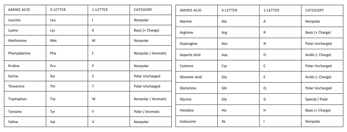
This article uses single letter codes. For example, the sequence of Trp-cage, one of the smallest stable folded proteins, is NLYIQWLKDGGPSSGRPPPS. This sequence consists of 20 amino acids. Different amino acid sequences have different lengths, typically ranging from 300 to 500 amino acids. Let L be the length of the input sequence. Then the input to the Alphafold 1 is a string of length L. For Trp-cage, L=20.

The output of Alphafold 1 is a sequence of torsion angles. For each amino acid in the input sequence, Alphafold 1 outputs two torsion angels, traditionally named 𝜙(phi) and ψ (psi). These torsion angles determine how the protein sequence folds in 3D space. For a sequence of length L, the output is a vector of length 2L. With the 40 torsion angles determined, the Trp-cage protein folds like this:

Folding visualization of Trp-cage from RCSB

Alphafold 1 workflow

Alphafold 1 consists of two components:

1. A convolutional neural network (CNN) that has two prediction heads. One head outputs a discrete distribution of distances between every pair of amino acids in the input protein sequence. This distribution describes the distance between the β-carbon atoms of an amino acid pair. The other prediction head outputs a discrete joint distribution of torsion angles (φᵢ, ψᵢ, hence joint) for each amino acid i in the input protein sequence. Please note that even though this neural network predicts torsion angles, those predicted torsion angles can be further improved. That’s why the Alphafold team included a second component.
2. An separate iterative optimization component finds the torsion angels (𝜙, ψ), such that when the protein folds according to the (𝜙, ψ) angles, the distance between every amino acid pair is as close as possible to the distances predicted by the convolutional neural network. In other words, this iterative optimization step uses the CNN predicted amino acid inter-distances as ground truth. It also uses the torsion angles predicted by the CNN as initial guess to kick the optimization started.

Now let’s go over these two components.

The convolutional neural network

The following figure shows the input and outputs of the convolutional neural network.

Input and outputs of the neural nework, by author

Convolutional neural network (CNN) is designed to process image image and produces output images. In our case, we can understand that the sequence and MSA features is an image of size L×L, where each pixel is a 478-channel vector. The input image captures first order information of the input sequence, which is information about amino acids at each of the i position, where i ∈ [1, L]. This image also captures second order information about every amino acid pair (i, j) at position i and j, where j ∈ [1, L].

The neural network’s first output is an L × L image-like representation. Each pixel at position (i, j) contains a 64-channel discrete probability distribution, where each channel represents the predicted likelihood that the distance between the amino acids at positions i and j falls within a specific distance bin.

The second output of the neural network is a 1D image of size L, each pixel represents a 1296-channel discrete probability distribution of the two torsion angles of each amino acid.

Neural network input

The inputs of the neural network is a L×L×487 tensor. Those 487 features for each amino acid pair consists of three parts:

1. Second order pairwise co-evolution strength features between every pair of amino acids, 21×21=441 in total.
2. First order amino acid features, 42 in total.
3. Auxiliary features, 4 in total.

I cover second order features before first order features because first order feature generation requires information acquired from second order feature generation.

Pairwise co-evolution strength features, 441 in total

Since the goal of the neural network is to predict the distance between every amino acid pair in the input sequence, it would make sense to find out whether an amino acid pair at position (i, j) is close to each other in naturally occurring protein sequences. To do that, Alphafold 1 searches for protein sequences that are similar to the input sequence databases.

Multiple sequence alignment

Genomic databases such as Uniclust30, BFD and UniRef90 contain millions of protein sequences with known folding structures. Alaphfold 1 uses sequence search tools such as HHblits or Jackhmmer to find sequences similar to the input sequence. The following figure illustrates the idea of finding similar sequences. Each letter in the table cells represents an amino acid, and a dash “-” means that there is gap amino acid. This gap is inserted by the search algorithm. The top row is the input sequence; the bottom three rows are similar sequences, one from sheep, one from chicken and the third from fish.

Multiple sequence alignment (MSA), by author

This is called a multiple sequence alignment (MSA) table. From this table, we can see that amino acids at position 1 and amino acids at position 4 co-evolve — when the position 1 amino acid change from A to B, the position 4 amino acid change from G to C. In other words, this is a correlated change.

Correlated changes at two amino acid positions across the sequences in a multiple sequence alignment (MSA) can provide evidence that the corresponding residues are in physical contact. When an amino acid at one position changes, interacting residues may also need to change to preserve the protein’s structural stability and overall three-dimensional shape. If these compensatory changes do not occur, the protein’s structure — and consequently its function — may be disrupted. Because natural selection tends to preserve mutations that maintain protein structure and function, pairs of positions that evolve in a correlated manner are more likely to be structurally or functionally related. But pleast note that such correlations do not always indicate a direct physical contact, as they may also arise indirectly through other interacting residues.

Alphafold 1 applies the Potts model on the multiple sequence alignment table and the input sequence to get a coupling parameter Jᵢ,ⱼ(a, b) for every amino acid pair (a, b) at position i and j. A larger Jᵢ,ⱼ(a, b) value means that the amino acid a at position i is more likely to be in contact with the amino acid b at position j.

Since there are 21 amino acids (20 real acids, plus one gap “-”). Jᵢ,ⱼ can be represented by a 21×21 matrix of shape 21×21:

Flatten this matrix to get the 441 co-evolution strength features.

First order amino acid features, 42 in total

This set of features encode the animo acid type at each position of the input sequence as well as the empirical probability distribution of all 21 amino acids at each location.

At position i, the amino acid type is encoded as an one-hot vector of length 21 (20 possible amino acids, plus a gap).

At position i, from the MSA table, compute the frequencies of amino acids at this position, which also results in a vector of length 21. For example, using the MSA table from above, we know:

• At position 1, the frequency of the amino acid A is: 1/3, and the frequency of the amino acid B is 2/3.
• At position 2, the frequency of the amino acid L is: 2/3, and the frequency of the gap is 1/3.
• And so on.

Then sum up these two 21-length vectors at each position to get the final vector at that position. Now we have a 1D feature matrix of shape L × 21. To expand this matrix into L × L, at each position pair (i, j), concatenate the 21-long 1D feature vector at position i and the 21-long 1D feature vector at position j, which results in a 42-long feature vector. For example, let Aᵢ and Aⱼ be the 1D feature vector at position i and j:

Then the concatenated 42-long feature vector for the position pair (i, j) is

Auxiliary features, 4 in total

Now the final 4 features. For every amino acid pair at position (i, j), the 4 auxiliary features are:

This will result in a L × L × 4 matrix.

The complete input matrix to the neural network is the concatenation of these three types of features along the feature dimension. Concatenating L × L × 441, L × L × 42 and L × L × 4 along the third dimension results in a matrix of shape L × L × 487.

Neural network outputs

The neural network has two outputs, the first is the inter amino acid distance distribution, and the other is joint torsion angle distribution.

Inter amino acid distance distribution

The predicted inter amino acid distance distribution is a L × L × 64 tensor. For an amino acid pair at position (i, j), a 64-dimensional discrete probability distribution is predicted. These 64 values sum up to 1 (via softmax) to form a proper probability distribution. Each value represents the probability that the distance between the β-carbon atoms of the amino acid at position i and position j falls in the a particular bin between 2 Å and 22 Å. Since there are 64 bins, each bin width is (22–2) / 64 = 0.3125 Å. The range of distance [2Å, 22Å] captures realistic distances between amino acid β-carbon atoms.

Distance between two amino acids at position (i, j) is symmetric. Inside the L × L × 64 tensor prediction, the 64-dimensional discrete distribution at location (i, j) should be equal to the distribution at location (j, i). To guarantee this property, Alphafold1 explicitly symmetrizes the network’s raw prediction before the softmax operation. Let the raw network output to be Y. We can understand Y is a square matrix of 64×64, and each entry in this matrix is a 64-dimensional vector. Alphafold 1 symmetrizes Y in the following way:

And then applies softmax on Y_sym along the channel dimension.

Joint torson angle distribution

The predicted joint torsion angle distribution is a L × 1296 tensor. For each amino acid at position i, the 1296-dimensional tensor represents the joint torsion angel 𝜙ᵢ, ψᵢ:

• Both the 𝜙ᵢ and ψᵢ angle range from -180° to +180°.
• AlphaFold 1 discretizes each angle into 10° equal-width bins, resulting in 36 bins per angle.
• Rather than predicting 𝜙ᵢ and ψᵢ independently with two separate 36-bin heads, the model predicts the joint distribution P(𝜙ᵢ, ψᵢ) across all possible combinations.

The advantage of predicting the joint distribution is to avoid invalid angle combinations if those angles are predicted independently. For example, if for an amino acid at position i, if 𝜙ᵢ = 120°, then ψᵢ can’t be 60°, a joint distribution can model this by predicting a low value for P(𝜙ᵢ=120°, ψᵢ=60°). If the two torsion angles are predicted independently, this kind of invalid correlation won’t be captured.

Neural network with fixed input size

Protein chains vary in lengths, different amino acids will have different length L. Even though convolutional neural networks can accepts varying length inputs, Alphafold 1 uses a CNN with the fixed input size 64 × 64 × 487. To handle an input amino acid sequence of length L, if L>64, Alphafold 1 first builds the L × L × 487 input matrix for the whole sequence. This L × L × 487 input matrix is a 487-channelled image of size L × L. Then Alphfold 1 produces 64 × 64 crops of this image and sends this crop to the neural network, as illustrated by the following figure.

Sliding window inference, from the Alphafold1 paper

During training, Alphafold 1 sends random crops of size 64×64 to the neural network. During inference, to avoid edging effect, Alphafold 1 uses overlapping sliding window inference. That is, it sends overlapping crops of size 64×64 to the network and averages the distance probability distributions for amino acids that appear in the overlapping crops.

If the input amino acid length L is shorter than 64, Alphafold 1 first creates a L×L×487 input matrix and then pads the matrix with zero values to create a 64×64×487 matrix. During training a single crop is used, and padding mask is used to make sure that padded entries do not contribute to loss calculation. During inference, the distance prediction of padded positions are ignored.

Training data

Alphafold1 uses 31,247 protein sequences, which were split into train and test sets (29,427 and 1,820 proteins, respectively) from the Protein Data Bank for training. Each training data point consists of an amino acid sequence and a distance matrix for each pair of amino acid in the sequence.

Loss of the neural network

Let dᵢ,ⱼ,ₖ be the discrete amino acid distance distribution prediction, where i, j ∈ [1, L] and k∈[1, 64] and Dᵢ,ⱼ,ₖ is the ground truth. Dᵢ,ⱼₖ is one-hot vector.

Let tᵢ,ₖ be the joint torsion angle discrete distribution prediction, where i ∈ [1, L] and k∈[1, 1296], and Tᵢ,ₖ is the torsion angle ground truth. Tᵢ,ₖ is a one-hot vector.

Then the loss of the neural network consists of two terms, one for the inter amino acid distance prediction and the other for the torsion angle prediction:

Optimizing input sequence torsion angles

The 2L amino acid torsion angles for the input protein sequence determines the 3D structure of the protein. As before, let (𝜙, ψ) be the torsion angles, with 𝜙 and ψ be vectors of length L.

In structural biology, there is a forward kinematics function x=G(𝜙, ψ), that returns the 3D coordinates of atoms in the protein sequence, with x being

where each xᵢ is a vector of the 3D coordinates of β-carbon atoms in the amino acid at position i. To simplify the explanation in this article, let’s treat xᵢ as the 3D coordinate of the β-carbon atom of the amino acid at position i. And we use the notation xᵢ=Gᵢ(𝜙, ψ) to represent that Gᵢ(𝜙, ψ) returns xᵢ.

Gᵢ(𝜙, ψ) is a function of 𝜙, ψ and is differentiable with respect to 𝜙 and ψ. This is important in the gradient descent optimization.

For two amino acids at position i and j, xᵢ=Gᵢ(𝜙, ψ) represents the 3D coordinate of the β-carbon atom of the amino acid at position i, and xⱼ=Gⱼ(𝜙, ψ) represents the 3D coordinate of the β-carbon atom of the amino acid at position j. Let dist(xᵢ, xⱼ) =|| xᵢ − xⱼ|| be the euclidean distance between these two 3D coordinates.

Now we have an analytical expression dist(xᵢ, xⱼ) that represents the distance between an amino acid pair at position (i, j), computed from torsion angles (𝜙, ψ). We can tweak the torsion angels to results in different inter amino acid distances. But how do we decide which torsion angles are the best? Remember that one of our neural network’s prediction is inter amino acid distance, so we can tweak the torsion angles such that the resulting dist(xᵢ, xⱼ) is as close to the corresponding neural network distance prediction as possible.

The neural network’s distance prediction is in the form of a 64-dimensional discrete distribution P(dᵢ,ⱼ | S, MSA(S)), where S is the input sequence and MSA(S) is the multiple alignment table for S. We can formulate the idea of dist(xᵢ, xⱼ) being close to neural network’s prediction as minimizing the following negative log likelihood, or alternatively, the potential function from the paper:

There is one problem, dist(xᵢ, xⱼ) returns a continuous value, but the network’s distance prediction is a discrete probability distribution. Also, using gradient descent to minimize this function requires this function to be fully differentiable with respect to 𝜙 and ψ.

We need to convert this discrete distribution into a differentiable continuous distribution. This is an easy task by using cubic spline interpolation. The result of applying cubic spline interpolation to a 64-dimensional discrete distribution is 63 cubic functions that connects these 64 values together. Each cubic function has the formula in the form of y=ax³ + bx² + cx + d, hence differentiable. The following chart illustrate cubic spline interpolation of 6 data points:

Cubic spline interpolation, by Google GEMINI

which results in the following fitted differentiable case function:

To differentiate this function with respect to x, first use the value of x to decide which case to use, and then following the normal differentiation rules.

Applying cubic spline interpolation to -log(P(dᵢ,ⱼ | S, MSA(S))) results in a fully differentiable negative log likelihood function with respect to torsion angles 𝜙 and ψ.

One last thing about this negative log likelihood. Raw log-probabilities suffer from background biases (e.g., amino acids in proteins are naturally constrained by chain connectivity and volume exclusion, even without specific evolutionary interactions. To overcome this, Alphafold 1 trains another neural network that predicts inter amino acid distance distributions only from the length of the input protein sequence. Denote this prediction as P(dᵢ,ⱼ | L). And we use this quantity to correct the original negative log likelihood:

Note that both log(P(dᵢ,ⱼ | S, MSA(S))) and log(P(dᵢ,ⱼ | L)) have cubic spline interpolation applied to turn them into differentiable continuous probability distributions.

Gradient descent via L-BFGS

Alphafold 1 uses the L-BFGS algorithm to find concrete 𝜙 and ψ torsion angles that minimizes the the negative log likelihood V_distance(𝜙, ψ) function. L-BFGS is an iterative numeric optimization method. It starts with an initial guess of the parameters (𝜙₀, ψ₀) and uses the gradient of the V_distance(𝜙, ψ) function to guide the direction of finding the next parameter values (𝜙₁, ψ₁), (𝜙₂, ψ₂) and so on to make the function smaller and smaller. Alphafold 1 uses the torsion angles predicted by the neural network as the initial angles (𝜙₀, ψ₀) for L-BFGS.

Other terms in the L-BFGS potential

The Alphafold 1 paper describes other terms in the L-BFGS potential function. These terms are included to produce better final predictions. Among all terms in the potential function, the previously defined V_distance(𝜙, ψ) is the most important term. Make sure you understand it. In Appendix, I will describe other terms for your interest.

Conclusion

This article explains the Alphafold 1 workflow. In the next two articles, I will cover Alphafold 2 and Alphafold 3.

Appendix: other terms in the potential function

Torsion potential energy term

Let (𝜙ₚ, ψₚ) denote the torsion angles predicted by the neural network. The torsion potential energy term encodes the idea that the optimized angles from the L-BFGS algorithm should be close to (𝜙ₚ, ψₚ). This makes sense, because it enforces that the neural network’s prediction is roughly correct (otherwise, why bother predicting them?), and restricts L-BFGS to fine-tune those predicted angles.

Let Pᵢ(a, b), i∈[1,L] denote the neural network predicted joint probability of torsion angle bin a and b for the i-th amino acid, a, b∈[1,36] because there are 36 bins for each angle with each bin having a width of 10°. a is the bin index for the torsion angle 𝜙ᵢ, b is the bin index for the torsion angle ψᵢ.

Let’s focus on the torsion angle 𝜙ᵢ. The marginal probability is:

Let θₐ=5 + (a-1)×10° be the mid-point angle in degrees of each of the 36 bins. Then compute the following weighted mean vectors on the unit circle:

With these mean vectors, estimate the following μ and R quantities:

Then we can define the following κ based on R:

Now we can define the von Mises probability density function:

This is a continuous probability distribution of an angle random variable 𝜙ᵢ defined on a circle, serving as the circular analogue to the standard normal distribution. 𝜙ᵢ ∈[0, 360°]. The μ quantity is the mean of this distribution and the κ quantity is the inverse of the variance. I₀ is defined as:

Please note I₀ doesn’t mention any torsion angles, its gradient is 0 with respect to torsion angles, hence can be ignored during the L-BFGS optimization.

Similar to the above, we can also define the probability density function for torsion angle ψᵢ:

Then the torsion potential energy term is defined as:

We can see that V_torsion is a joint negative log likelihood for all the torsion angles 𝜙 and ψ, evaluated using the von Mises probability distribution. The shape (that is, the means μ and the inverse of the variance κ) of these von Mises probability distributions are empirically estimated from the torsion angles predicted by the neural network. Minimizing this term encourages the optimal torsion angles to be close to what the neural network predicts.

The following table describes the impact of R on the V_torsion optimization.

The score2_smooth term

V_score2_smooth(𝜙, ψ) is a term from the Rosetta work. This term add further physical constrains over the optimized torsion angles 𝜙 and ψ. If you are interested, please find more details of this term. For the purpose of this article, it is sufficient to know that the V_score2_smooth(𝜙, ψ) is also differentiable with respect to 𝜙, ψ.

The final loss function for L-BFGS to minimize