GEOSPATIAL ANALYSIS I KNIME I STORIES

Finding Pharmacy Deserts: A Geospatial Analysis with KNIME

How to combine isodistance polygons with census grid data to identify underserved areas in Germany

Working with geodata is one of the most rewarding tasks for a data scientist — there is almost always a beautiful visualization waiting at the end. And KNIME Analytics Platform with its Geospatial Analytics Extension makes handling the peculiarities of geospatial data remarkably easy.

But what if you need geodata to answer a real policy question? In Germany, a proposed pharmacy reform law would allow pharmacies to operate with reduced staffing and equipment requirements — provided they are established in areas more than 6 km road distance from the nearest existing pharmacy. This immediately raises a concrete analytical question: which areas in Germany are more than 6 km road distance from the nearest pharmacy, how many square kilometers do they cover, and how many people live there?

In collaboration with the *Deutsche Apotheker Zeitung*, we investigated this question using a geospatial workflow in KNIME. This article walks you through the analytical approach, demonstrating three key capabilities: preparing and transforming geodata from different sources, using spatial joins and set operations to identify areas without pharmacy coverage, and visualizing multi-layer geospatial results. A demo workflow with a reduced dataset is available on the KNIME Hub — we’ll link it at the end.

The figure below shows the complete workflow. For demonstration purposes, we use a reduced dataset covering only a small region. The full analysis for all of Germany follows the same logic.

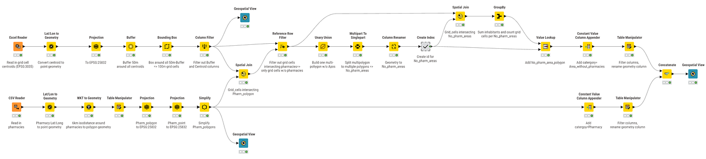
Fig. 1. The complete KNIME workflow for the pharmacy distance analysis

From Raw Coordinates to Analysis-Ready Geometries

Any geospatial analysis starts with getting the data into the right shape. In our case, we had two datasets to prepare.

For the full analysis, the first is a proprietary dataset of all pharmacies in Germany with geocoordinates — close to 17,000 locations. The second is the freely available Census 2022 grid data, which covers Germany at a resolution of 100 × 100 m. For each grid cell, the census provides a centroid coordinate and a population count. In total, this amounts to approximately 3 million grid cells — or 3 million rows in our table.

The pharmacy data: isodistance polygons via API. For the pharmacies, a simple point on the map is not enough. We need the 6 km road distance zone around each location — the isodistance polygon. We used the Mapbox Isochrone API for this, sending GET requests for all pharmacies directly from KNIME. The API allows 300 requests per minute, so we had the isodistance polygons for all ~17,000 pharmacies within about an hour. We stored these polygons as WKT (Well-Known Text) so they could be read and written via CSV files. The demo workflow uses a subset of these results for a small region. The analytical steps, however, are the same.

The census data: reconstructing grid cells from centroids. Let’s look at the upper path in the workflow. The census grid centroids arrive with coordinates in EPSG:3035. We first convert them to point geometries using the Lat/Lon to Geometry node, then project them to EPSG:25832 using the Projection node. EPSG:25832 is optimized for distance calculations in Germany.

However, point geometries are not enough — we need the full 100 × 100 m grid cells for our spatial analysis. Here we apply a neat trick: we create a 50 m Buffer around each centroid, then apply a Bounding Box to each buffer. The bounding box of a circle with 50 m radius is a square with exactly 100 m side length. This effectively reconstructs the original grid cells around each centroid.

Fig. 2. Census grid cells (blue squares) reconstructed from centroids using the buffer and bounding box method. Each cell covers 100 × 100 m. The area shown is around Karlsruhe.

Preparing the pharmacy polygons. The lower path in the workflow handles the pharmacy data. First, the Lat/Lon to Geometry node creates point geometries from the pharmacy coordinates. Then the WKT to Geometry node converts the stored isodistance strings into polygon geometries. Both are projected to EPSG:25832 using Projection nodes. Finally, the Simplify node applies a very light simplification to the polygon edges — this speeds up the subsequent spatial join without noticeably affecting accuracy.

At this point, our two datasets are ready: the census grid cells as square polygons and the pharmacy isodistance zones as irregular polygons. Visualizing the pharmacy isodistance polygons in a Geospatial View already gives us an idea of the coverage:

Fig. 3. Pharmacy isodistance polygons (blue) showing the 6 km road distance zones. Gaps in the coverage are clearly visible.

Identifying Areas Without Pharmacy Coverage

With both datasets prepared, the core analytical step is a Spatial Join. This node joins the pharmacy isodistance polygons with the census grid cells using the “intersects” match mode: every grid cell that is touched by at least one pharmacy’s 6 km zone appears in the result table.

But we are interested in the opposite: the grid cells that are not covered by any pharmacy. To get these, we use the Reference Row Filter node to remove all matched grid cells from the original dataset. What remains are the cells more than 6 km road distance from any pharmacy. In our demo dataset, 144 grid cells survive this filter.

These individual grid cells often form contiguous areas. To identify coherent regions, we apply two operations in sequence. First, the Unary Union node merges all 144 remaining grid cells into one large multipolygon. Then, the Multipart to Singlepart node splits this multipolygon into separate, connected polygons — each representing a distinct area without pharmacy coverage. In our demo data, this yields 31 separate areas.

Now we need to calculate the population for each of these areas. We assign an index to each area using a Create Index metanode. This index is essential for what follows: we join these 31 areas back with the individual grid cells using another Spatial Join, then use a GroupBy node to sum up the inhabitants for each area index. Finally, the Value Lookup node reattaches the polygon geometries to our aggregated data.

The result is a table showing each underserved area with its polygon geometry, the number of grid cells it contains, and the total population.

A note for the KNIME developers: It would be helpful if the Spatial Join node could retain all join columns. Currently, at least one geometry column is lost in the process, which requires the Value Lookup workaround described above.

Visualizing Multi-Layer Geospatial Results

The ideal visualization would display two layers on a single map: the pharmacy isodistance polygons in one color and the underserved areas in another. Currently, both the Geospatial View node and the Kepler.gl Geoview node in KNIME can only process one geometry column at a time. Another note for the KNIME developers: Supporting multiple geometry columns in a single view would be a welcome enhancement for future versions.

Until then, there is a practical workaround. We merge the two geometry columns into a single column and add a “Category” column to distinguish between the two types: “Pharmacy” for the isodistance zones and “Area_without_pharmacies” for the underserved regions. By concatenating the rows from both datasets — each tagged with its category we can visualize everything in one Geospatial View with color-coded categories.

The resulting map clearly shows the 6 km isodistance zones around pharmacies alongside the areas that fall outside any pharmacy’s reach. The dark blue areas represent the zones within 6 km of a pharmacy. The red squares are the individual census grid cells representing inhabited areas more than 6 km road distance from any pharmacy.

Zooming in reveals the details. Each underserved region can be clicked to display its attributes, including the population count. This gives a direct, visual answer to the policy question: where exactly are the gaps, and how many people are affected?

Fig. 4. Geospatial View showing pharmacy isodistance zones (blue) and underserved areas with inhabited grid cells (red squares) on a single map. The tooltip shows 898 inhabitants living more than 6 km from the nearest pharmacy.

Of course, the visual exploration is only one way to use these results. By sorting a GroupBy node output in descending order by population, we can immediately identify which contiguous areas without pharmacy coverage have the most inhabitants — and therefore represent the most promising candidates for new pharmacy locations. And since each grid cell covers exactly 0.01 km², summing up the cells per area also gives us the size of each underserved region in square kilometers. This turns the analysis from a purely descriptive map into a prioritized list for decision-makers.

Geodata Meets Policy Analysis

This workflow demonstrates how KNIME’s geospatial nodes — from coordinate transformations and buffer operations to spatial joins and polygon merging — can turn raw location data into actionable policy insights. By combining pharmacy isodistances with census population data, we identified the specific areas and population counts affected by the proposed reform. Applied to the full dataset, the analysis reveals that nearly 5 million people in Germany currently live outside the 6 km road distance zone of any pharmacy — and that about 15% of Germany’s settled area falls outside this zone.

The approach is transferable to many similar questions: wherever you need to assess the spatial coverage of services — whether pharmacies, hospitals, schools, or public transport — the same pattern of isodistance calculation, spatial joining, and set operations applies.

The demo workflow is available on the KNIME Hub for you to explore and adapt.