Prediction Intervals vs Confidence Intervals

Photo by Logan Voss on Unsplash

We’ve all heard of confidence intervals, but in practice, prediction intervals are often more useful, and much easier for stakeholders to understand.

What Are Confidence Intervals?

When we fit a model to a dataset, we assume the dataset is only a sample from the full population. If we were to draw a different sample and fit the same model again, the estimated parameters would usually be different. This means the fitted model is uncertain.

Take a simple linear regression as an example. Imagine repeatedly drawing samples from the same population and fitting a regression line each time. The fitted lines will not be identical. They will vary from sample to sample.

A confidence interval (CI) quantifies this variability. It is constructed so that, if we repeatedly sample from the population and build a confidence interval each time, about 95 out of 100 of those intervals would contain the true population parameter. You can find an excellent visualisation here.

Each parameter of the model has its own confidence interval. For example, the slope has a 95% CI, and the intercept has a 95% CI.

Why is this useful? Across repeated samples, some confidence intervals will miss the true parameter, but most will capture it. The width of the confidence interval tells us how variable our parameter estimates are. Higher variability in the data leads to wider confidence intervals.

How to Calculate Confidence Intervals (Bootstrap Method)

One practical way to calculate confidence intervals is using bootstrapping:

1. Create a bootstrap sample from the dataset (sampling with replacement).
2. Fit the model to the bootstrap sample and record the model parameters.
3. Repeat steps 1 and 2 for N times (for example, 400 times).
4. For each parameter, you now have 400 values. Take the 2.5th and 97.5th percentiles.
5. These percentiles form the lower and upper bounds of the 95% confidence interval.
6. Repeat this for all model parameters.

Why Confidence Intervals Are Not Enough

Confidence intervals describe the uncertainty of the fitted model, not the range of actual outcomes.

In real data, there are always residuals, which are the differences between predicted values (ŷ) and true values (y). Even if the model were perfectly known and exactly matched the population relationship, individual predictions would still vary because of random noise. Real data points will not fall exactly on the predicted line.

The range that captures both model uncertainty and residual noise is called the prediction interval.

A Very Simple House Price Example

Imagine you build a model to predict house prices based on size, location, and age of the house.

You use past sales data to fit the model.

Confidence Interval: Uncertainty About the Model

Suppose your model predicts that a particular house is worth $500,000.

A 95% confidence interval might say:

Based on the data, the average market price of this type of house is between **$480,000 and $520,000**.

What this means:

• The interval describes uncertainty in the model’s estimate of the average price.
• If you repeatedly collected new datasets and refit the model, about 95% of those confidence intervals would contain the true average price for this type of house.
• This interval is about the model, not about a specific sale.

Prediction Interval: Uncertainty About Real Outcomes

Now think about what actually happens in the real world.

Two identical houses can sell for very different prices because of negotiation, buyer preferences, timing, and random market factors.

A 95% prediction interval might say:

This house is likely to sell for somewhere between **$420,000 and $580,000**.

What this means:

• The interval describes where an individual house price is likely to fall.
• It includes both uncertainty in the model, and natural variability in real house prices.
• Even with a perfect model, individual sales would still vary.

If a buyer asks, “What is this house worth?” They usually care about worst-case and best-case outcomes, not the uncertainty of your regression coefficients.

That’s why prediction intervals are usually wider, but more useful.

How to Calculate Prediction Intervals

Prediction intervals extend the bootstrap idea by explicitly accounting for residuals:

1. Fit the model to the original dataset and record the residuals.
2. Create a bootstrap sample from the dataset.
3. Fit the model to the bootstrap sample and record the predicted values (ŷ).
4. For each predicted value, randomly add one residual from the original model.
5. Repeat steps 2–4 for N times (for example, 400 times).
6. For each observation, you now have hundreds of simulated predictions that include noise.
7. Take the 2.5th and 97.5th percentiles of those predictions.
8. These percentiles form the 95% prediction interval for that observation.

Implementation of CI and PI Without Bootstrap

# Confidence vs Prediction Intervals (simple demo)
# Uses a built-in sklearn dataset (diabetes), fits a simple linear regression
# and visualises:
#   - 95% Confidence Interval for the mean prediction (CI)
#   - 95% Prediction Interval for a new observation (PI)

import numpy as np
import matplotlib.pyplot as plt

from sklearn.datasets import load_diabetes
import statsmodels.api as sm

# ----------------------------
# 1) Load a built-in dataset
# ----------------------------
data = load_diabetes(as_frame=True)
df = data.frame.copy()

# Predict disease progression (target) from BMI only
x = df["bmi"].to_numpy()
y = df["target"].to_numpy()

# ----------------------------
# 2) Fit linear regression with statsmodels
# ----------------------------
X = sm.add_constant(x)  # add intercept
model = sm.OLS(y, X).fit()

print(model.summary())

# ----------------------------
# 3) Create a smooth x-grid for plotting intervals
# ----------------------------
x_grid = np.linspace(x.min(), x.max(), 200)
X_grid = sm.add_constant(x_grid)

# get_prediction returns both:
#  - mean confidence interval (for E[y|x])
#  - observation/prediction interval (for a new y at x)
pred = model.get_prediction(X_grid).summary_frame(alpha=0.05)

y_hat = pred["mean"].to_numpy()

# 95% CI for the mean response
ci_low = pred["mean_ci_lower"].to_numpy()
ci_high = pred["mean_ci_upper"].to_numpy()

# 95% PI for a new observation
pi_low = pred["obs_ci_lower"].to_numpy()
pi_high = pred["obs_ci_upper"].to_numpy()

# ----------------------------
# 4) Visualise
# ----------------------------
plt.figure(figsize=(10, 6))

# scatter of the raw data
plt.scatter(x, y, s=18, alpha=0.35, label="Data")

# fitted line
plt.plot(x_grid, y_hat, color="black", linewidth=2, label="Fitted line")

# confidence interval band (narrower)
plt.fill_between(x_grid, ci_low, ci_high, color="dodgerblue", alpha=0.25,
                 label="95% Confidence interval (mean)")

# prediction interval band (wider)
plt.fill_between(x_grid, pi_low, pi_high, color="orange", alpha=0.18,
                 label="95% Prediction interval (new observation)")

plt.title("Confidence vs Prediction Intervals (Linear Regression)")
plt.xlabel("BMI (standardized)")
plt.ylabel("Disease progression target")
plt.legend()
plt.grid(True, alpha=0.25)
plt.tight_layout()
plt.show()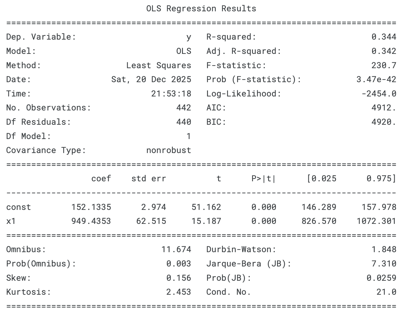

This example uses the diabetes dataset from scikit-learn. It contains medical measurements for a group of patients, along with a target variable that measures disease progression one year later.

To keep things simple and easy to visualise, the model uses:

• BMI as the only input feature
• Disease progression as the target

We fit a linear regression using statsmodels, which gives us direct access to analytical confidence intervals and prediction intervals. Once the model is fitted, we create a smooth range of BMI values and ask the model to predict outcomes across that range.

What the Confidence Interval Represents

The confidence interval shown in the plot is the 95% confidence interval for the mean response:

If many patients had this BMI, where would the average disease progression likely fall?

The CI reflects uncertainty in the estimated regression line, which comes from limited sample size and variability in the data.

What the Prediction Interval Represents

The prediction interval is the 95% interval for a single new observation:

For one new patient with this BMI, how much could the outcome realistically vary?

The prediction interval includes uncertainty in the fitted model and natural variability in individual outcomes (residual noise).

Why We Do Not Need Bootstrap Here

For linear regression models fitted with statsmodels, both confidence intervals and prediction intervals can be computed directly using closed-form statistical formulas. These intervals rely on classical assumptions such as linearity, independent errors, and approximately normally distributed residuals, and they are available out of the box for multiple linear regression.

For most other models, confidence and prediction intervals are usually estimated using bootstrap methods.

Implementation of CI and PI With Bootstrap

# Bootstrap Confidence vs Prediction Intervals (simple demo)
# Uses a built-in sklearn dataset (diabetes), fits a simple linear regression
# and visualises bootstrap-based:
#   - 95% Confidence Interval for the mean prediction (CI)
#   - 95% Prediction Interval for a new observation (PI)

import numpy as np
import matplotlib.pyplot as plt

from sklearn.datasets import load_diabetes
import statsmodels.api as sm

# Reproducibility
rng = np.random.default_rng(42)

# ----------------------------
# 1) Load a built-in dataset
# ----------------------------
data = load_diabetes(as_frame=True)
df = data.frame.copy()

# Keep it simple: predict disease progression (target) from BMI only
x = df["bmi"].to_numpy()
y = df["target"].to_numpy()
n = len(y)

# ----------------------------
# 2) Fit the "core" model on the original data (to get residuals)
# ----------------------------
X = sm.add_constant(x)  # add intercept
core_model = sm.OLS(y, X).fit()

y_hat_core = core_model.predict(X)
residuals = y - y_hat_core

# ----------------------------
# 3) Create a smooth x-grid for plotting intervals
# ----------------------------
x_grid = np.linspace(x.min(), x.max(), 200)
X_grid = sm.add_constant(x_grid)

# ----------------------------
# 4) Bootstrap CI and PI
# ----------------------------
B = 400  # number of bootstrap resamples (keep modest for speed)

# Store bootstrap draws for:
# - mean predictions (for CI)
# - "new observation" predictions with residual noise (for PI)
boot_mean_preds = np.empty((B, len(x_grid)))
boot_obs_preds = np.empty((B, len(x_grid)))

for b in range(B):
    # (a) Resample rows (pairs bootstrap)
    idx = rng.integers(0, n, size=n)
    x_b = x[idx]
    y_b = y[idx]

    X_b = sm.add_constant(x_b)
    model_b = sm.OLS(y_b, X_b).fit()

    # (b) Mean prediction on the grid from this bootstrap-fitted model
    mean_pred_b = model_b.predict(X_grid)
    boot_mean_preds[b, :] = mean_pred_b

    # (c) Add residual noise to approximate new observations (prediction interval)
    # We sample residuals from the *core* model to keep the noise level anchored
    eps = rng.choice(residuals, size=len(x_grid), replace=True)
    boot_obs_preds[b, :] = mean_pred_b + eps

# 95% intervals from bootstrap percentiles
ci_low, ci_high = np.percentile(boot_mean_preds, [2.5, 97.5], axis=0)
pi_low, pi_high = np.percentile(boot_obs_preds, [2.5, 97.5], axis=0)

# Also plot the core fitted line
y_hat_grid = core_model.predict(X_grid)

# ----------------------------
# 5) Visualise
# ----------------------------
plt.figure(figsize=(10, 6))

plt.scatter(x, y, s=18, alpha=0.35, label="Data")
plt.plot(x_grid, y_hat_grid, color="black", linewidth=2, label="Fitted line (core model)")

plt.fill_between(
    x_grid, ci_low, ci_high,
    color="dodgerblue", alpha=0.25,
    label="95% Bootstrap CI (mean)"
)

plt.fill_between(
    x_grid, pi_low, pi_high,
    color="orange", alpha=0.18,
    label="95% Bootstrap PI (new observation)"
)

plt.title("Bootstrap Confidence vs Prediction Intervals (Linear Regression)")
plt.xlabel("BMI (standardized)")
plt.ylabel("Disease progression target")
plt.legend()
plt.grid(True, alpha=0.25)
plt.tight_layout()
plt.show()

Using the same dataset as above. We still fit a linear regression using statsmodels, but this time we use bootstrap resampling to compute both confidence intervals and prediction intervals.

The idea is to simulate what would happen if we repeatedly collected “new” datasets from the same population by resampling the original data (with replacement). For each bootstrap sample, we refit the model and predict across a smooth range of BMI values.

What the Confidence Interval Represents

In the bootstrap version, we generate many fitted lines by refitting the model on many bootstrap samples. For each BMI value on the grid, we collect the predicted values across all bootstrap runs and take the 2.5th and 97.5th percentiles. That percentile band is the bootstrap CI. It reflects how much the estimated regression line changes due to sampling variability.

What the Prediction Interval Represents

After each bootstrap-fitted model produces a prediction, we add a randomly sampled residual (taken from the residuals of the core model fitted to the original dataset). This produces “noisy” predictions that mimic the spread of actual outcomes. Taking the 2.5th and 97.5th percentiles of these noisy predictions gives the bootstrap PI.

Key Takeaways

Confidence intervals answer: “How uncertain is the model?”

Prediction intervals answer: “How much can reality vary?”

Confidence intervals are always narrower because they ignore individual-level variability. For linear regression, CI and PI can be computed analytically; for most other models, bootstrap methods are the practical solution.

The code I used in this blog post can be found here.